Two Infinities
Sun, 04 Apr 2021
Speckle Interferometry
The autocorrelogram provides an intuitive explanation of speckle analysis, but Fourier analysis provides a framework for inverse filtering (deconvolution) as developed by Labeyrie in 1971. Here is a look at a model and an example.
Part 1: Model
The idea starts out the same in both views. Namely the observed image I is the sum of several images, each the diffraction limited image O having passed through a different cell of air with its own refractive index resulting in a shift of O by a random vector u_j. (Following the Teχ convention of using the underscore to indicate a subscript and letting n denote the number of images.)
I = (1/n)Σ_j O * δ_(u_j), j = 1...n
That is, under the assumption of shift invariance and non-distortion, I is the convolution product of the system input image with the point spread function (PSF), the output image of a point source, here expressed as an equally weighted sum of delta functions.
The Fourier transform of I, F(I), is linear,
F(I) = (1/n)Σ_j F( O * δ_(u_j))
and the transform of a convolution product is the point product of the transforms,
F(I) = (1/n)F(O) ∙ Σ_j F( δ_(u_j))
and the transform of the delta function is the plane wave,
v → exp( -i ∙ v • u_j), v ∈ ℝxℝ
where the bold dot (•) indicates the vector inner product. So taking just the modulus squared of the Fourier transform,
|F(I)|²(v) = (1/n)²|F(O)|²Σ_(j,k) exp(-i · v • (u_j - u_k)), j,k = 1...n,
the product of the transformed input image with the modulation transfer function (MTF). When j = k, the summand equals 1. For the n(n-1) summands where j ≠ k, a real-valued interference term is obtained, cos(v • (u_j - u_k)). If the u_j are independent normal random vectors with variance σ², then the expected value of cos(...) is exp(-|v|²σ²).
If numerous images are captured and the distributions remain stationary, then the images may be averaged. Then, assuming v constrained by the frequency limit of the telescope, by the law of large numbers,
<|F(I)|²(v)> ≈ |F(O)|²(1/n + ((n-1)/(2n))exp(-|v|²σ²))
as the number of samples increases.
Special cases. If n = 1, then the MTF is simply 1, of course. For n > 1, the MTF is a sum of a constant and a Gaussian. If n = 2, then the MTF is
1/2 + exp(-|v|²σ²)/4
And if n = 3, then the MTF is
1/3 + exp(-|v|²σ²)/3
As n increases, that is, the more refracting cells and choppy the air, the balance shifts from the constant to the exponential. As σ² increases, the variance of the Gaussian, proportional to the reciprocal of σ², decreases. Both have the effect of bunching the system response into lower frequencies and suppressing the higher, hence limiting angular resolution.
If O were simply a point source, then looking in the space domain, it's autocorrelation, ideally a single point, would be partially obscured by interference among the speckles, represented here as linear combination of δ₀ and a Gaussian with mean 0 and variance now proportional to σ².
Now suppose that image O is the sum of two point sources, like a double star, say one point at the origin and the other at point w, δ_0 and δ_w with Fourier transforms constant 1 and plane wave v → exp(-2πiv•w). The power spectral density is then
2 + exp(-2πiv•w) + exp(2πiv•w) = 2 + 2cos(2πv•w)
which when transformed back to autocorrelation becomes the triple sum of delta functions
2δ_0 + δ_w + δ_(-w)
Thus, in the presence of speckle noise, we have in the frequency domain
v → (2 + 2cos(2πv•w))(1/n + ((n-1)/(2n))exp(-|v|²σ²))
and taking the inverse transfrom, one recovers the two star autocorrelation with Gaussian noise added in, possibly enough to obscure the relative maxima of the autocorrelation. Of course, if this PSF were a good guide to actual observation, one could use the MDF to construct an inverse filter.
Labeyrie's approach to the PSF was suggested by star photographs and Kolmogorov's model for atmospheric turbulence. Starting there, astronomers have developed more sophisticated models. For example, Jack Drummond has developed a model of the PSF as a sum of a Bessel function and the Cauchy distribution. (Thanks to R. Q. Fugate for the reference).
Part 2: Example of inverse filtering, STF 848
Data: 25 images of double star STF848 (Henry Draper 41943), each exposed for 5 milliseconds each. Here is an animated GIF of the first fifteen (refresh to run again):
We take these images and compute their autocorrelatograms and average them together, essentially checking to see whether the triple of delta functions above can be distinguished through the noise:
Suggestive perhaps but actually nothing pops out; there is only one local maximum.
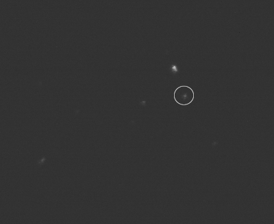
So, following Labeyrie, we try an inverse filter, one where the filter divisor is obtained by approximating the PSF. The double star STF 848 sits in the "37" open cluster in Orion, and our images contain additional stars in the same frame. In particular STF 848 itself is assigned a visual companions. STF 848D, magnitude 8.3, is circled here in the first frame of our set; STF 848 A and B comprise the bright blob above it:
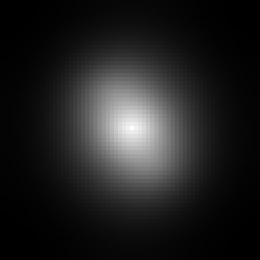
Using the 25 exposures to compile an average MTF for STF 848D, we construct the unassuming composite:
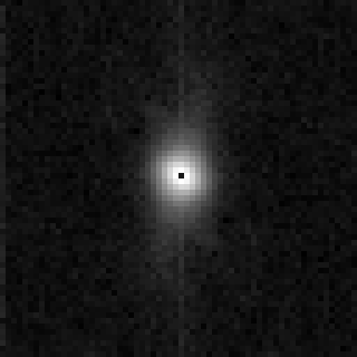
However, when we compute the element-wise quotient of the average STF 848AB MTF by the average STF 848D MTF and then take the inverse Fourier transform back to the spacial domain to obtain the filtered autocorrelogram, we get this:
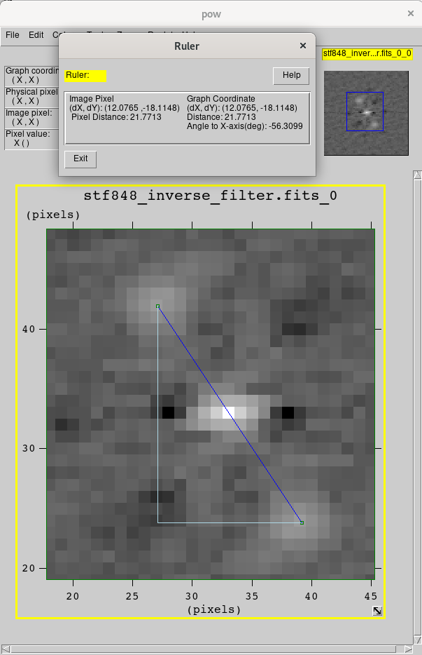
where suddenly the triple peaks of a double star autocorrelogram can be detected.
Using the ruler tool in the fv FITS viewer for instance, the side peaks are found to be about 21.77 pixels apart. The instrument used here has a focal length of 82 inches and the camera has 2.4 μm wide pixels, hence about .238 arcseconds per pixel. Thus 21.77 px translates to 2.587" separation between STF 848 A and B stars. The "precise separation" listed at Stelle Doppie is 2.605" for agreement within .1" with our estimate.
Scientists have developed many filtering techniques including blind deconvolution using the model above and Gaussian speckle-masking described by A. W. Lohman et al, 1983, (thanks to D. Elmore for introduction to speckle masking) when no reference star is available.
posted at: 11:58 | path: | permanent link to this entry
