Two Infinities
Sun, 06 Jul 2025
STELAR group at Mt Wilson Observatory
This report is a slice of data acquired Thursday, May 22, 2025 with the Hooker 100" telescope on Mt Wilson.
Richard Bell operated the telescope. Target stars were selected by Leon (and Nick remotely) using the NINA plugin. Reference stars were selected by NINA from a list provided by Tom S. The list of targets was developed in cooperation with Russ: multi-peak fraction < 80 on Thursday, multi-peak fraction > 80 on Wednesday. Filter selection was guided by Geoff who provided autocorrelation images from the first 100 exposures of the targets.
The first goal was to estimate what portion of Gaia 2-parameter astrometric solution stars are multiple stars. Back in November, Geoff had identified a possible triple system from October observations, and in response to a question about the system, Cécile Loup of SIMBAD had said "There is no astrometric solution in Gaia DR2 nor DR3 [for TYC 2761-582-1], which probably means that this star is double." The idea was to estimate what that probability might be.
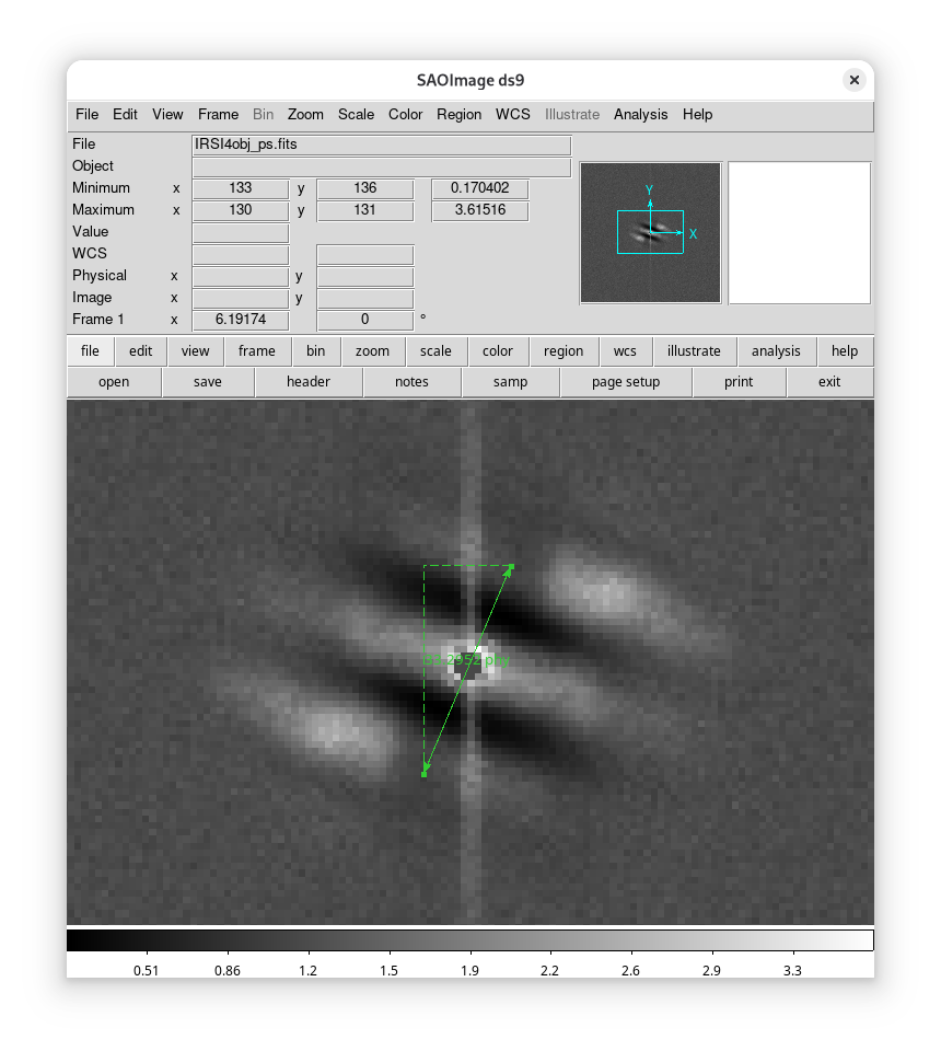
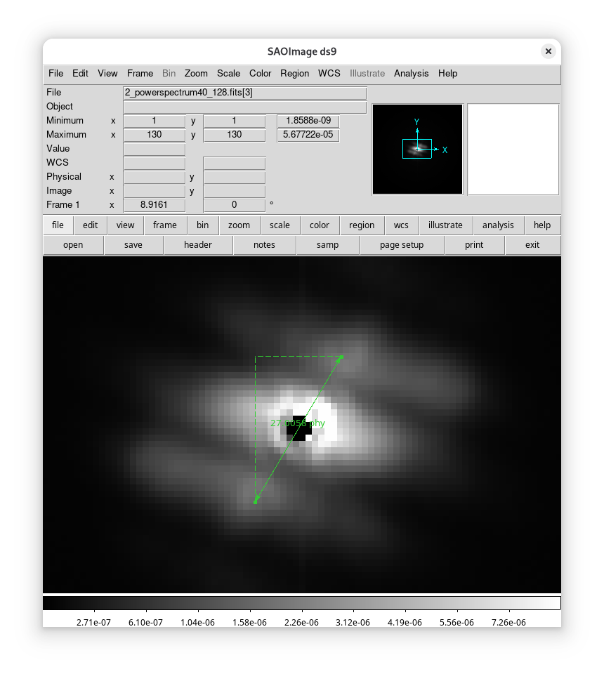
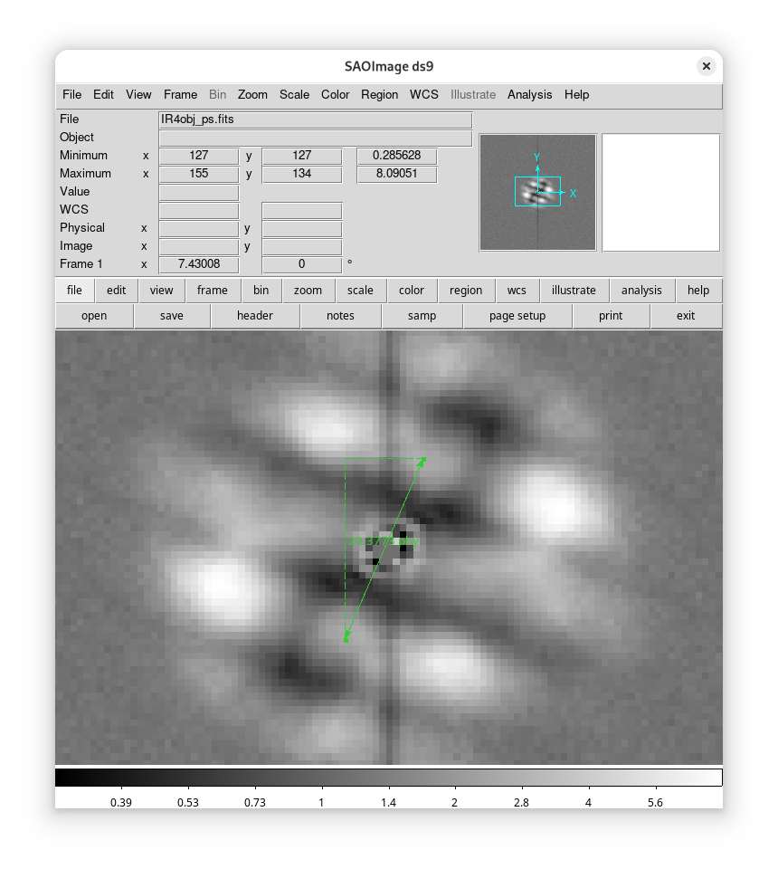
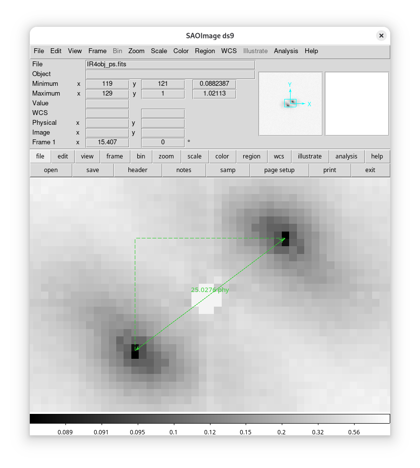
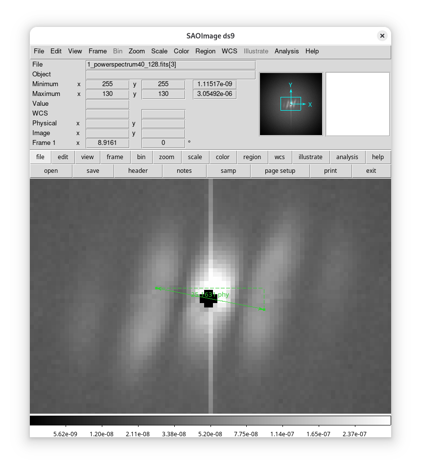
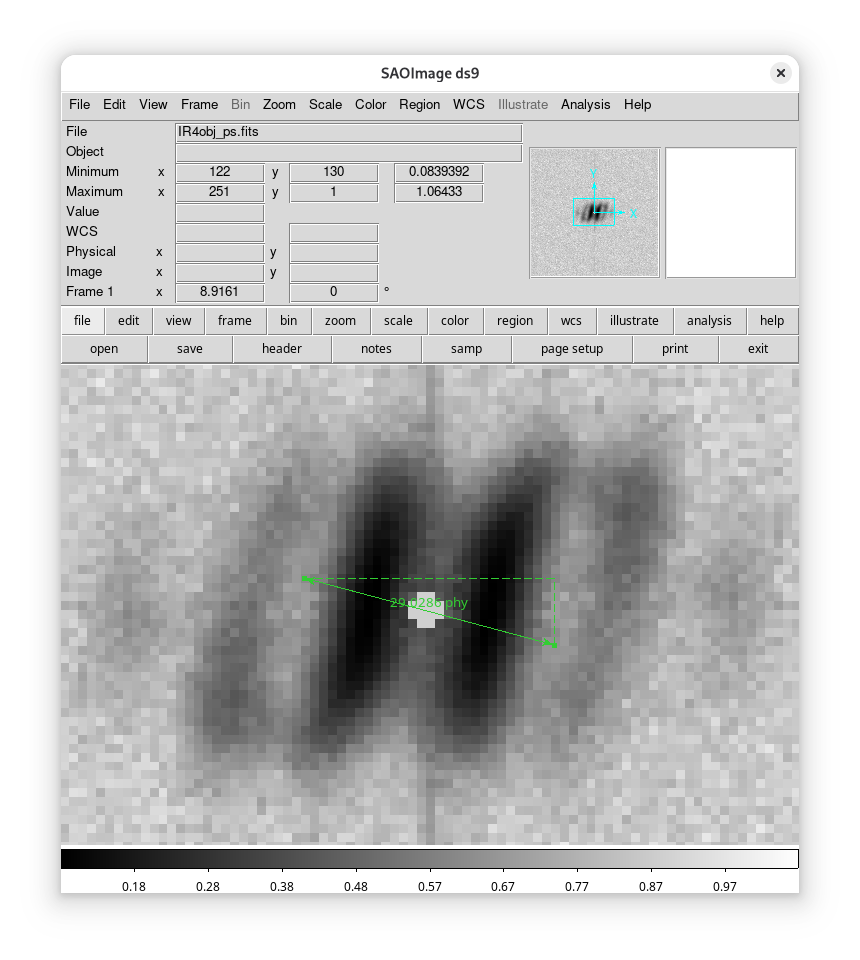
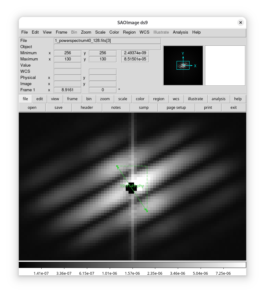
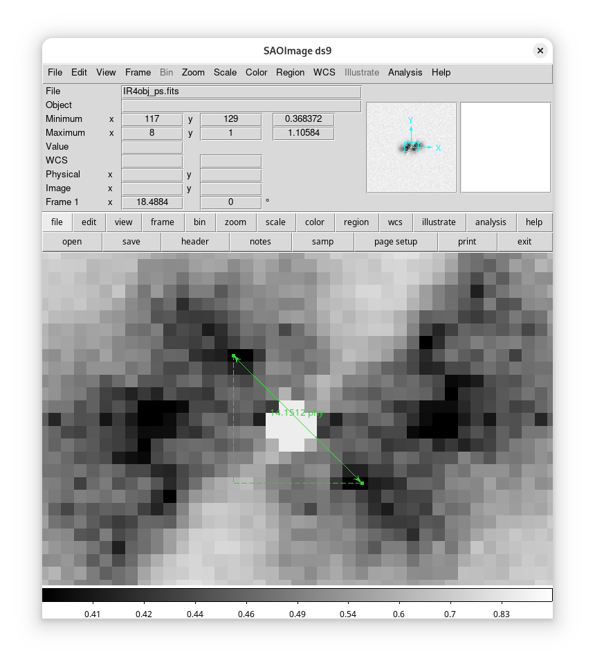
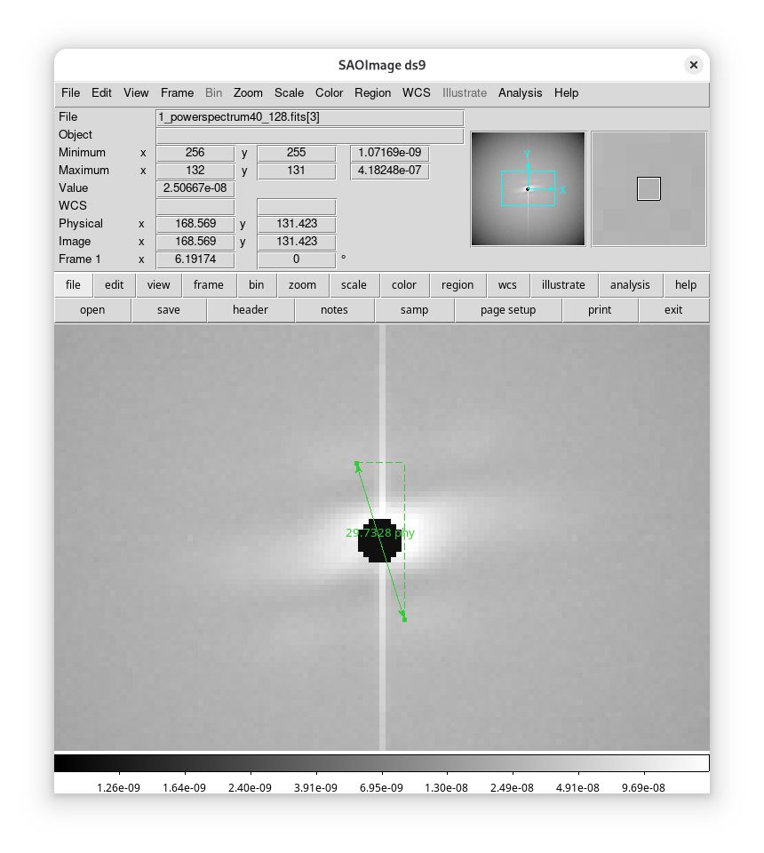
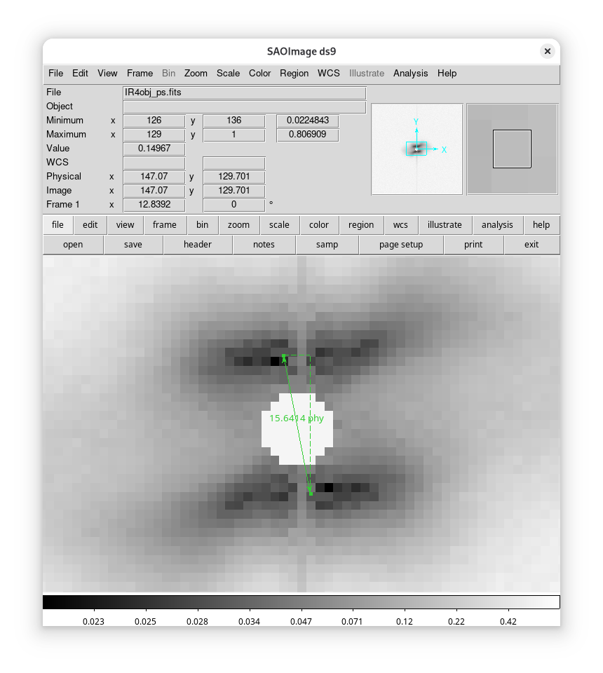
It turned out that each of our targets exhibited signs of multiplicity. Some quite obvious; others less so. Separations were roughly measured to be between about 0.1 and 0.3 arcseconds based on a plate scale estimated at 0.0117 arcseconds/pixel. More precise results may be available from Geoff's bispectrum reductions using Dave's Speckle Toolbox.
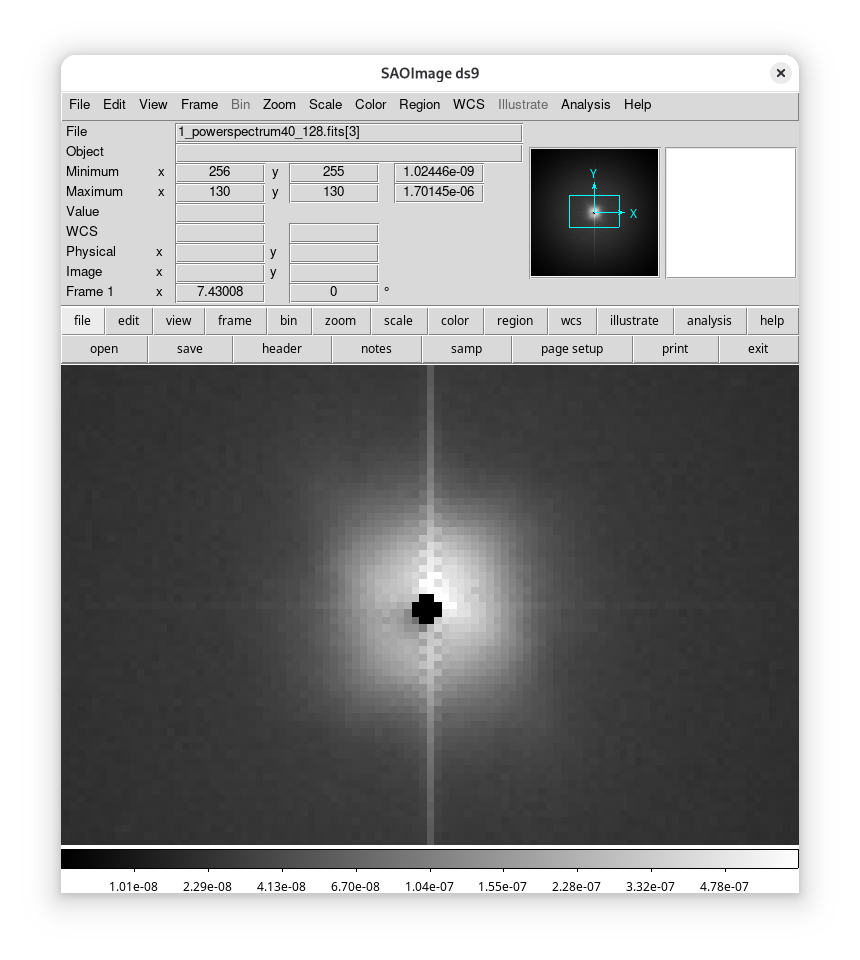
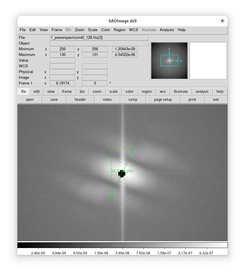
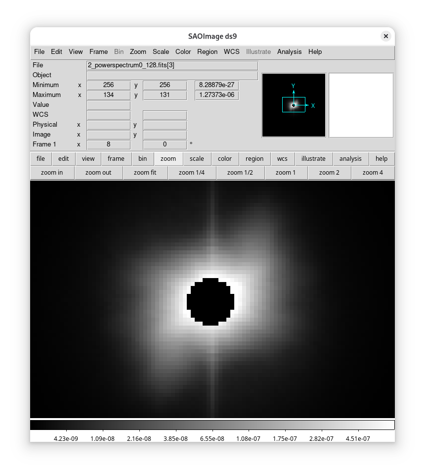
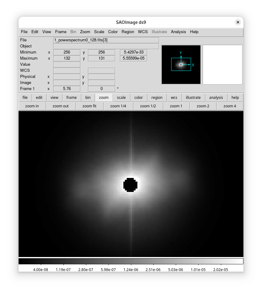
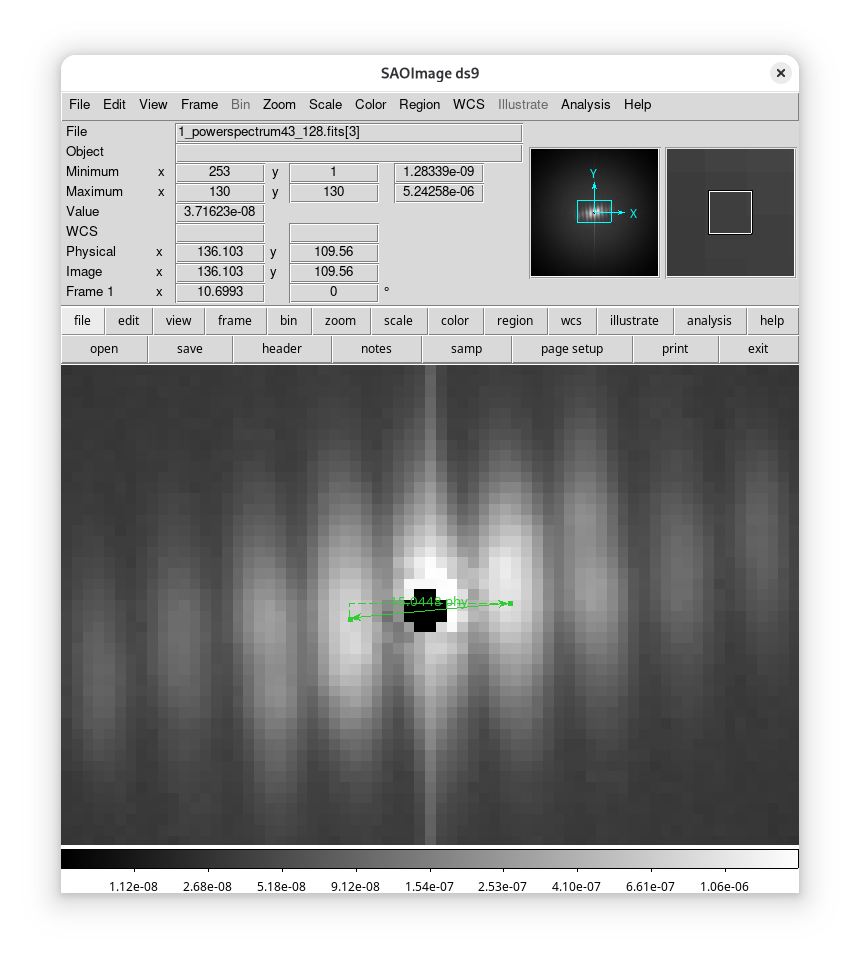
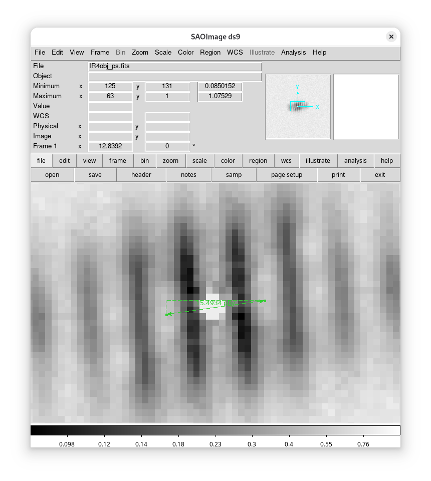
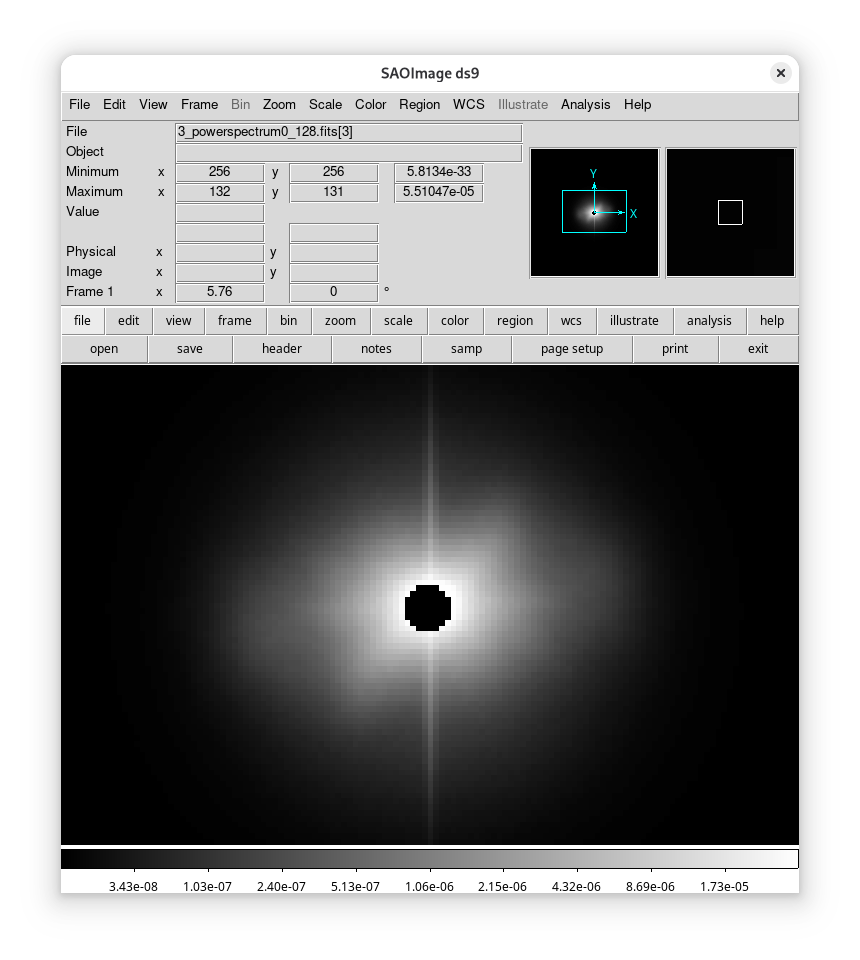
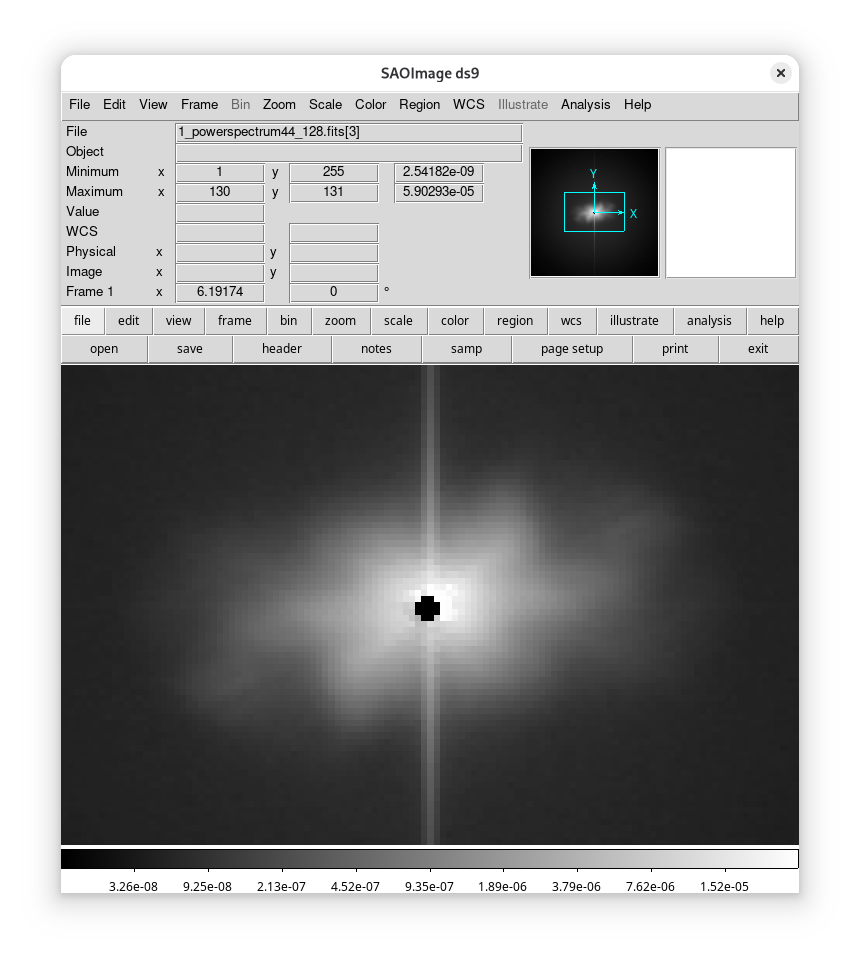
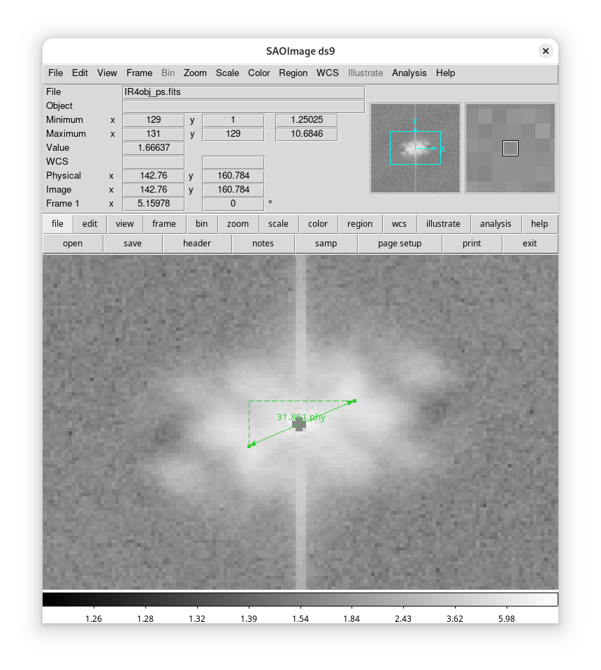
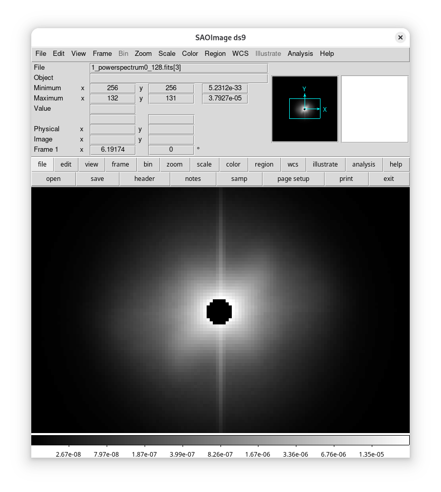
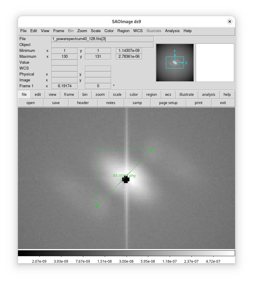
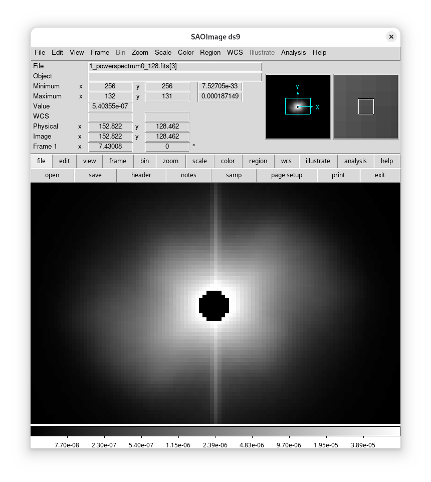
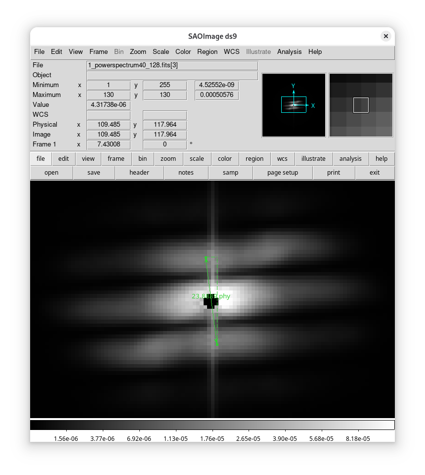
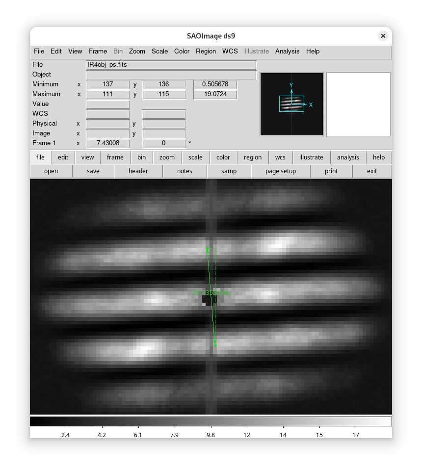
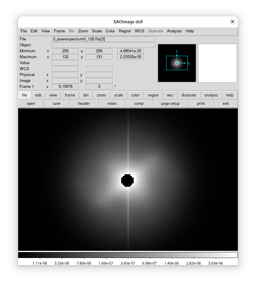
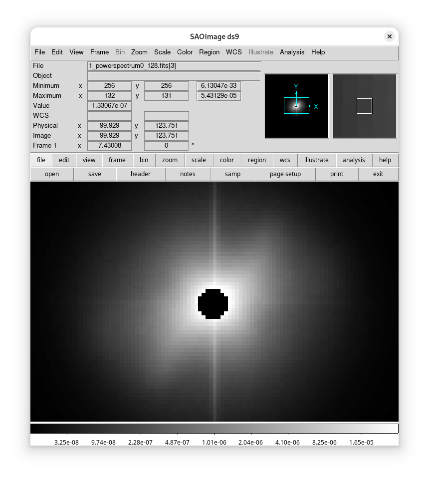
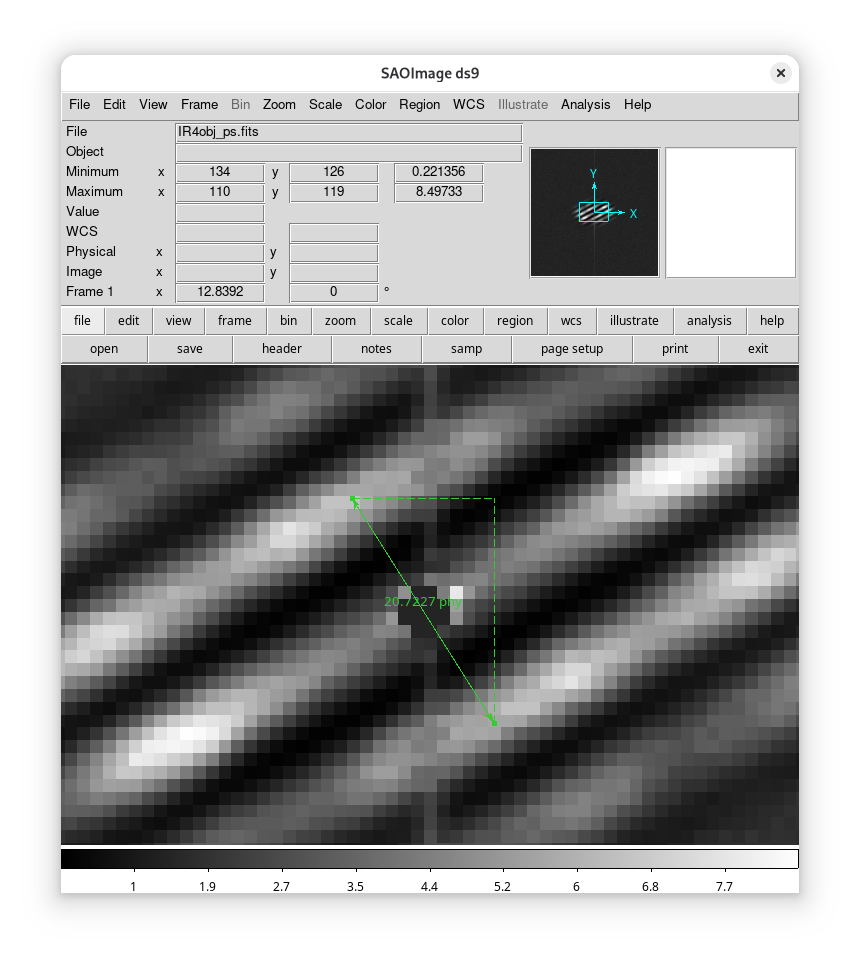
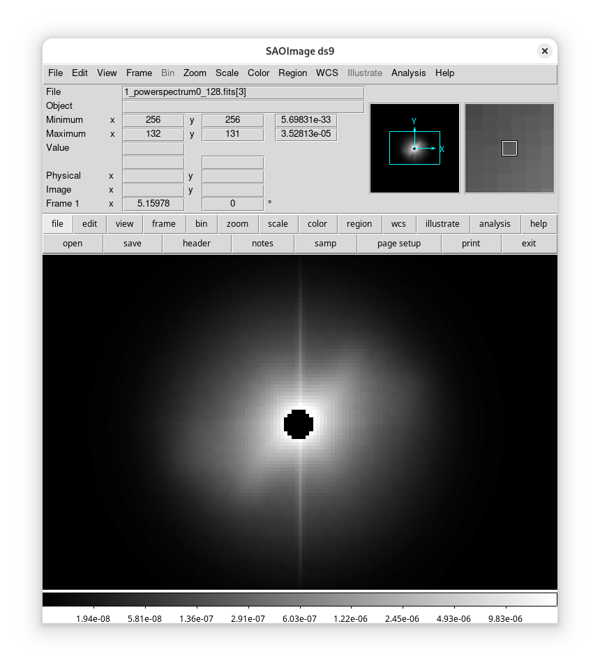
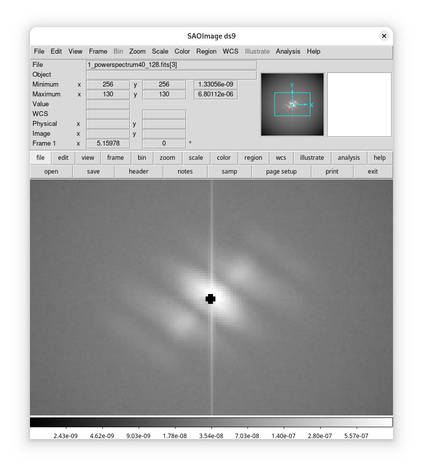
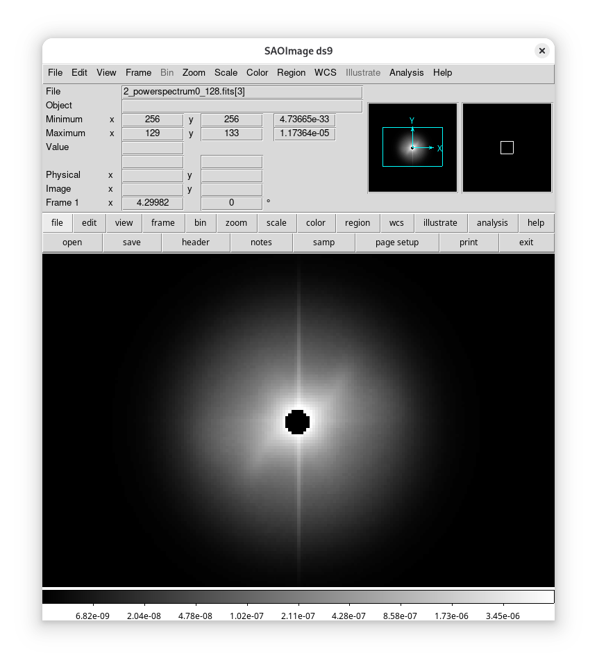
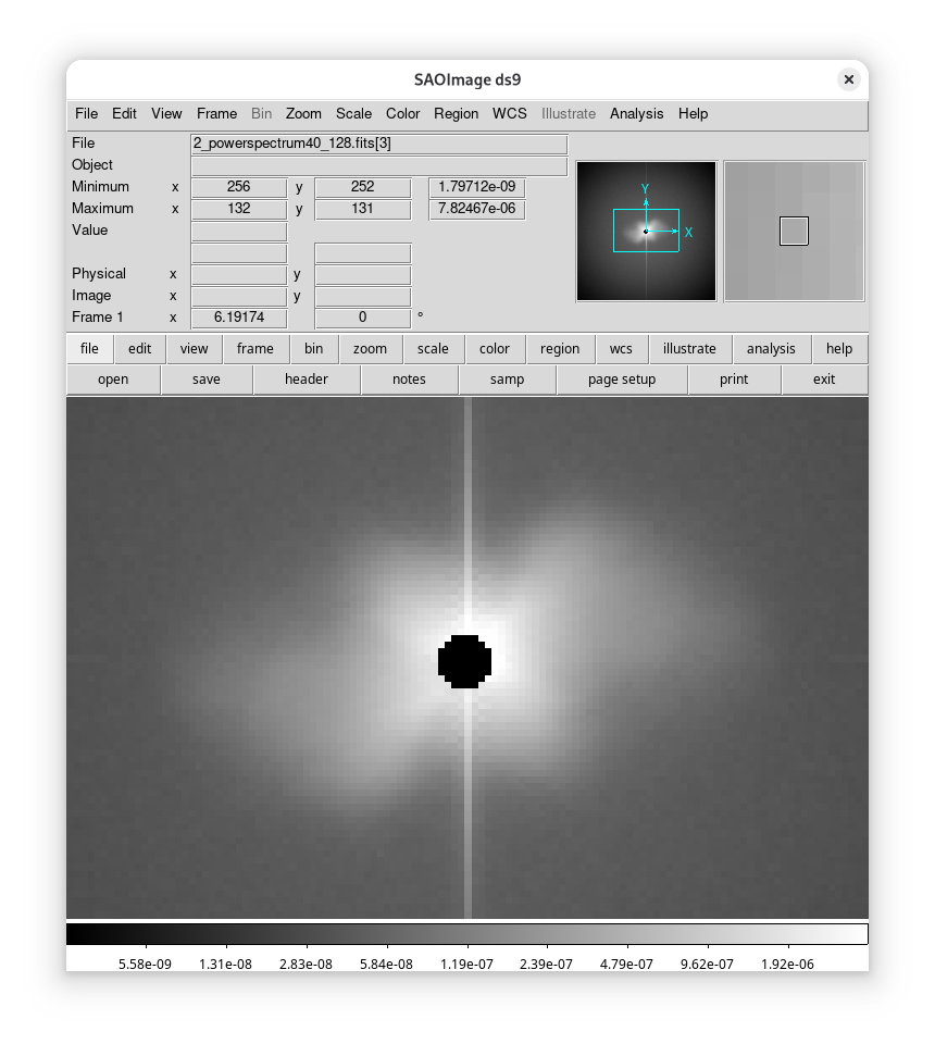
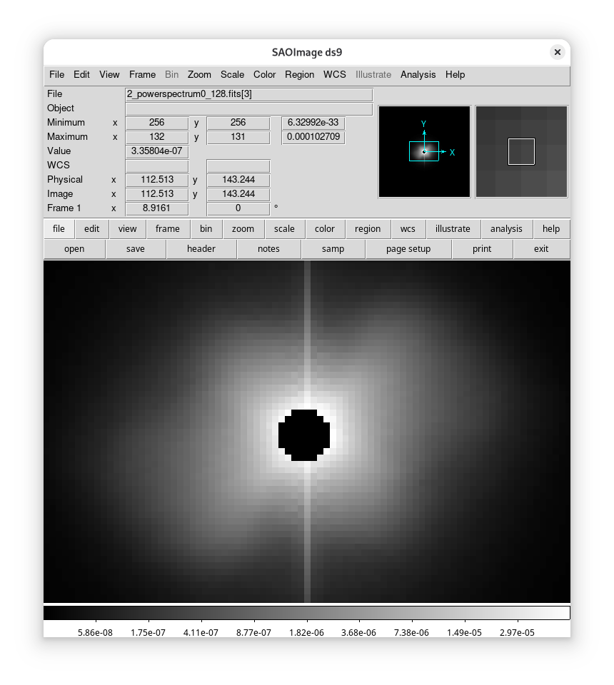
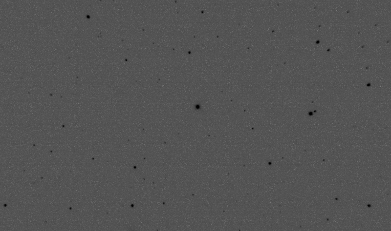
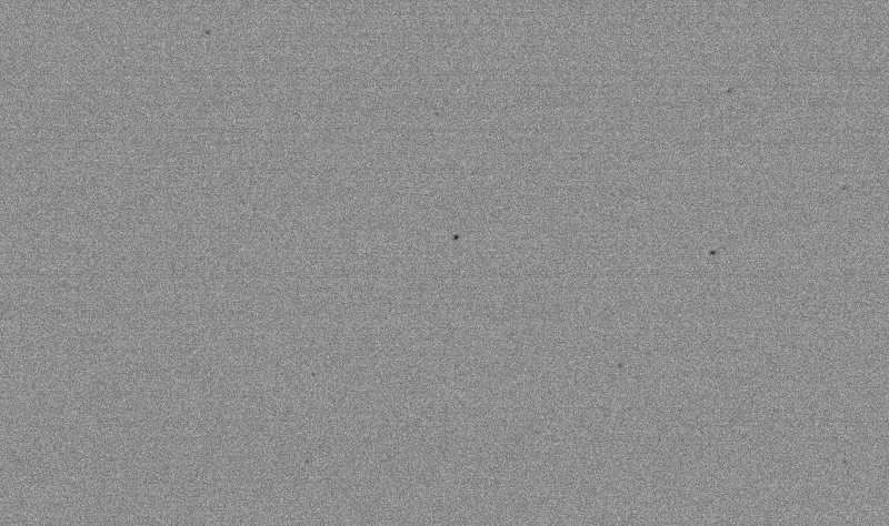
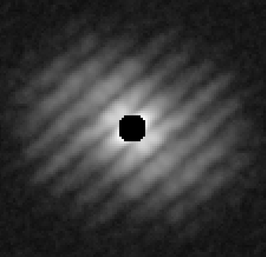
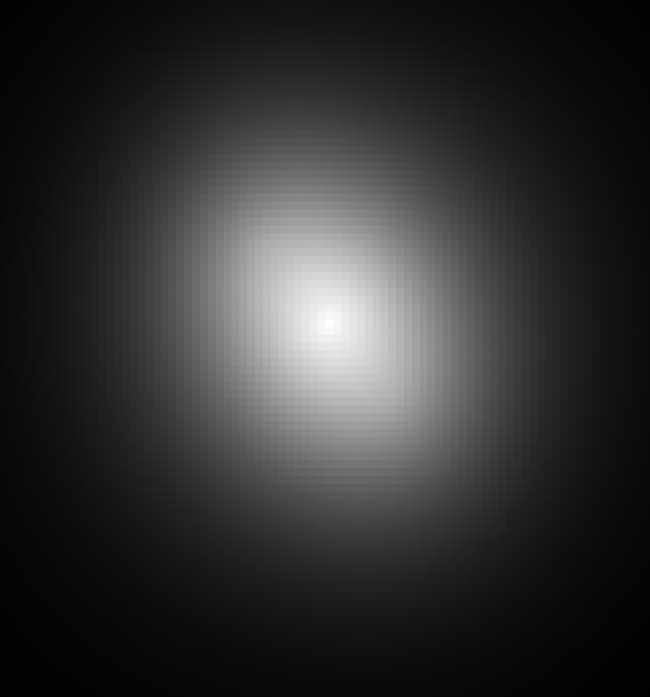
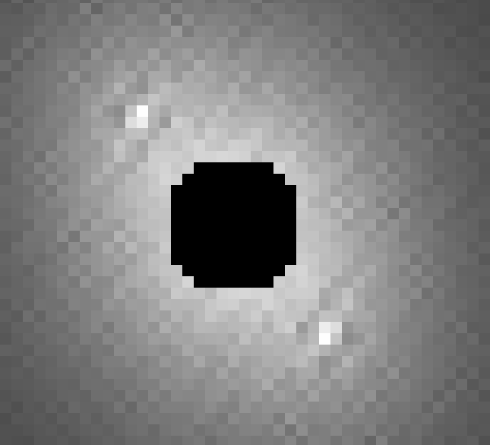
Three images are displayed for each target: first the power spectrum of the reference star, second the power spectrum of the target, and third the quotient of the target power spectrum by the reference power spectrum à la Labeyrie. All images were taken through the IR-pass filter except for the first reference star where the Sloan I filter was used.
The parallactic angle of each target star at time of observation was computed to guard against any obvious distortion by atmospheric refraction. Such refraction must occur given the non-zero zenith angles and the wide bandwidth of the IR-pass filter, but it did not appear to affect the first order approximations.
Lastly, a summary of filters and exposures used is tabulated along with filters with which fringes were detected and the range of measured separations for filters and methods.
Filters
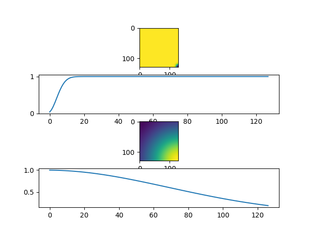
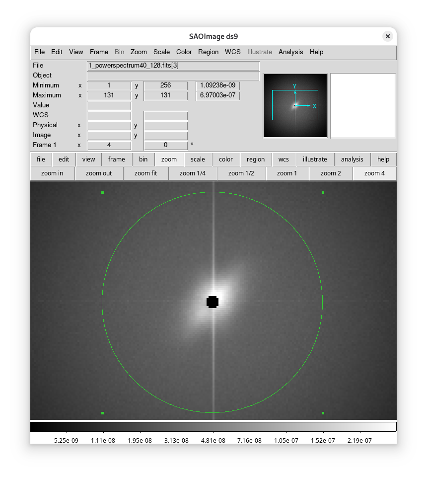
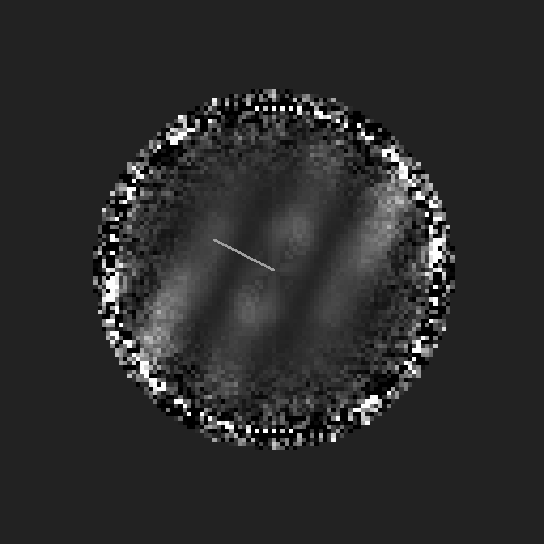
Gaussian high pass and low pass filter profiles. Theoretical resolution limit occurs at about 52.7 pixels out. See the circle in the G2PS193 power spectrum below.
G2PS010
G2PS018
G2PS055
G2PS078
G2PS102
G2PS120
G2PS132
G2PS161
G2PS179
G2PS193
G2PS209
| Target | RA | Dec | source_id | Gmag | FDBL | GOFHA | BREX |
|---|---|---|---|---|---|---|---|
| str7 | float64 | float64 | int64 | float64 | int64 | float64 | float64 |
| G2PS010 | 185.14 | 30.60 | 4013740572694929408 | 10.29 | 71 | 0.31 | 67.54 |
| G2PS015 | 187.27 | 9.53 | 3903824800447407232 | 11.35 | 44 | 0.20 | 11.92 |
| G2PS018 | 189.90 | 31.95 | 1514419835236108032 | 9.50 | 56 | 0.17 | 21.23 |
| G2PS019 | 190.00 | 11.16 | 3928344150265115520 | 11.34 | 25 | 0.21 | 2.08 |
| G2PS055 | 202.89 | 11.20 | 3738443614381976448 | 10.34 | 53 | 0.14 | 43.08 |
| G2PS078 | 208.67 | 12.82 | 3728535399707693696 | 9.10 | 1 | 0.02 | 4.23 |
| G2PS102 | 214.11 | 19.89 | 1252031418311733120 | 10.51 | 39 | 0.16 | 11.17 |
| G2PS120 | 218.37 | 26.57 | 1280208735939184000 | 6.19 | 47 | 0.25 | 47.26 |
| G2PS132 | 222.69 | 22.26 | 1265524006532379392 | 10.92 | 57 | 0.39 | 58.84 |
| G2PS161 | 231.83 | 18.08 | 1208848889404284416 | 8.19 | 73 | 0.29 | 106.01 |
| G2PS179 | 235.27 | 16.69 | 1196966295444346368 | 9.94 | 64 | 0.35 | 42.10 |
| G2PS193 | 238.63 | 15.12 | 1193174354721344384 | 10.62 | 47 | 0.24 | 8.59 |
| G2PS209 | 243.18 | 22.07 | 1205620826343661696 | 11.24 | 40 | 0.21 | 23.03 |
| G2PS215 | 245.24 | 7.43 | 4451820571100096640 | 11.19 | 35 | 0.13 | 6.38 |
| Target | obstime | sidereal | HA | p-angle |
|---|---|---|---|---|
| deg | deg | |||
| str7 | Time | float64 | float64 | float64 |
| G2PS010 | 2025-05-23T03:38 | 177.62 | -7.52 | 13.73 |
| G2PS015 | 2025-05-23T03:56 | 182.00 | -5.26 | 24.60 |
| G2PS018 | 2025-05-23T04:41 | 193.30 | 3.39 | -6.05 |
| G2PS019 | 2025-05-23T04:16 | 187.04 | -2.97 | 12.75 |
| G2PS055 | 2025-05-23T05:11 | 200.96 | -1.94 | 8.37 |
| G2PS078 | 2025-05-23T05:34 | 206.70 | -1.97 | 7.63 |
| G2PS102 | 2025-05-23T06:01 | 213.33 | -0.78 | 2.09 |
| G2PS120 | 2025-05-23T06:18 | 217.75 | -0.62 | 1.29 |
| G2PS132 | 2025-05-23T06:36 | 222.26 | -0.43 | 1.04 |
| G2PS161 | 2025-05-23T07:09 | 230.59 | -1.24 | 3.59 |
| G2PS179 | 2025-05-23T07:23 | 233.89 | -1.38 | 4.28 |
| G2PS193 | 2025-05-23T07:34 | 236.75 | -1.88 | 6.34 |
| G2PS209 | 2025-05-23T07:58 | 242.79 | -0.39 | 0.94 |
| G2PS215 | 2025-05-23T07:52 | 241.19 | -4.05 | 23.21 |
| Target | filt_ir_exp | filt_lu_exp | filt_sg_exp | filt_sr_exp | filt_si_exp |
|---|---|---|---|---|---|
| s | s | s | s | s | |
| str7 | float64 | float64 | float64 | float64 | float64 |
| G2PS010 | 0.06 | 0.04 | -- | -- | -- |
| G2PS015 | 0.14 | 0.08 | -- | -- | -- |
| G2PS018 | 0.06 | 0.04 | -- | -- | -- |
| G2PS019 | 0.09 | 0.06 | -- | -- | -- |
| G2PS055 | 0.06 | 0.04 | 0.06 | 0.06 | 0.06 |
| G2PS078 | 0.06 | 0.04 | 0.06 | 0.06 | 0.06 |
| G2PS102 | 0.06 | 0.04 | -- | -- | -- |
| G2PS120 | 0.02 | 0.02 | 0.06 | 0.06 | 0.06 |
| G2PS132 | 0.06 | 0.04 | -- | -- | -- |
| G2PS161 | 0.03 | 0.02 | 0.02 | -- | -- |
| G2PS179 | 0.06 | 0.04 | -- | -- | -- |
| G2PS193 | 0.06 | 0.04 | -- | -- | -- |
| G2PS209 | 0.09 | 0.06 | 0.06 | 0.06 | 0.06 |
| G2PS215 | 0.09 | 0.06 | 0.06 | -- | -- |
posted at: 14:05 | path: | permanent link to this entry
Wed, 01 May 2024
Speckle Interferometry Background and Example
Presented to Enchanted Sky Star Party October, 2023.
Light
Astronomers study light.
wave propagation
Christiaan Huygens

superposition
Thomas Young diffraction and interference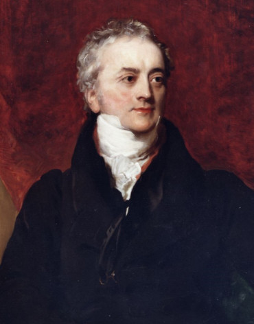

(painting by Henry Perronet Briggs)
speed of light differs with media
The different media might be different densities of air. Different speeds lead to refraction (Fermat's principle).
Pierre de Fermat
Laser refracted by ultrasound

Poisson's spot
Arguing against Augustin Fresnel's wave theory of light, Siméon Denis Poisson claimed there would have to be a tiny bright spot in the middle of the defocused image of a star in a telescope with central obstruction. When, contrary to Poisson's expectation, such a spot did occur, many scientists were won over to the theory. (Image from Suiter's "Star Testing".)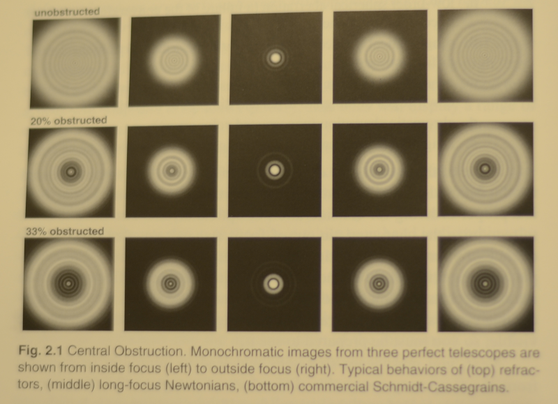
X-ray chrystalography
The periodicity of electro-magnatic radiation is useful for delineating the periodic structure of chrystals -- most famously for uncovering the structure of DNA: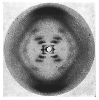
Basic Idea
Same Image Viewed Two Different Ways
Joseph Fourier proposed that any function can be viewed as the superposition of cyclic functions. For example, instead of viewing an image as an array of pixel values, view it as a superposition of waves. If a good approximation of the function can be obtained with a few waves then the change of point of view reveals structure.
![]()
Averaging Out Atmospheric Turbulence
Antoine Labeyrie thesis, extension of Fizeau and Michelson's interferometer methods:

Quote: "Speckle" refers to the grainy structure observed when a laser beam is reflected from a diffusing surface.
Labeyrie snippets courtesy J. Briggs' book from Yerkes library.
Binary Star Example
cou1333: Constellation Cygnus, Tycho2 2702-00556-1
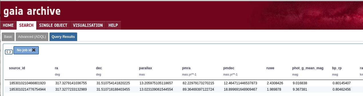
From parallax the distance from Earth is about 247 light years. From ruwe each star probably has a companion; that is, this double is probably physical.
Go to Astropy to compute the angular separation between Gaia coordinates.
#!/usr/bin/env python3
import sys
import astropy.units as u
from astropy.coordinates import SkyCoord

# usage: angle_sep.py 〈ra1 〉 〈dec1 〉〈ra2 〉〈dec2 〉 (in degrees)
# output: angular separation in arcseconds
ra1 = float(sys.argv[1])
dec1 = float(sys.argv[2])
ra2 = float(sys.argv[3])
dec2 = float(sys.argv[4])

c1 = SkyCoord(ra1*u.deg, dec1*u.deg, frame='fk5')
c2 = SkyCoord(ra2*u.deg, dec2*u.deg, frame='fk5')
sep = c1.separation(c2)
print('angular separation',sep.arcsecond)
Run the script like this:
./angle_sep.py 317.3279141036755 31.510754141820225 317.3277233132989 31.510718188403455Get the result in arcseconds:
angular separation 0.599698853444346
Pixels to Angles
Getting from pixels to arcseconds.
Using Plate Solve
Using astrometry.net solve-field, the plate solution for this image: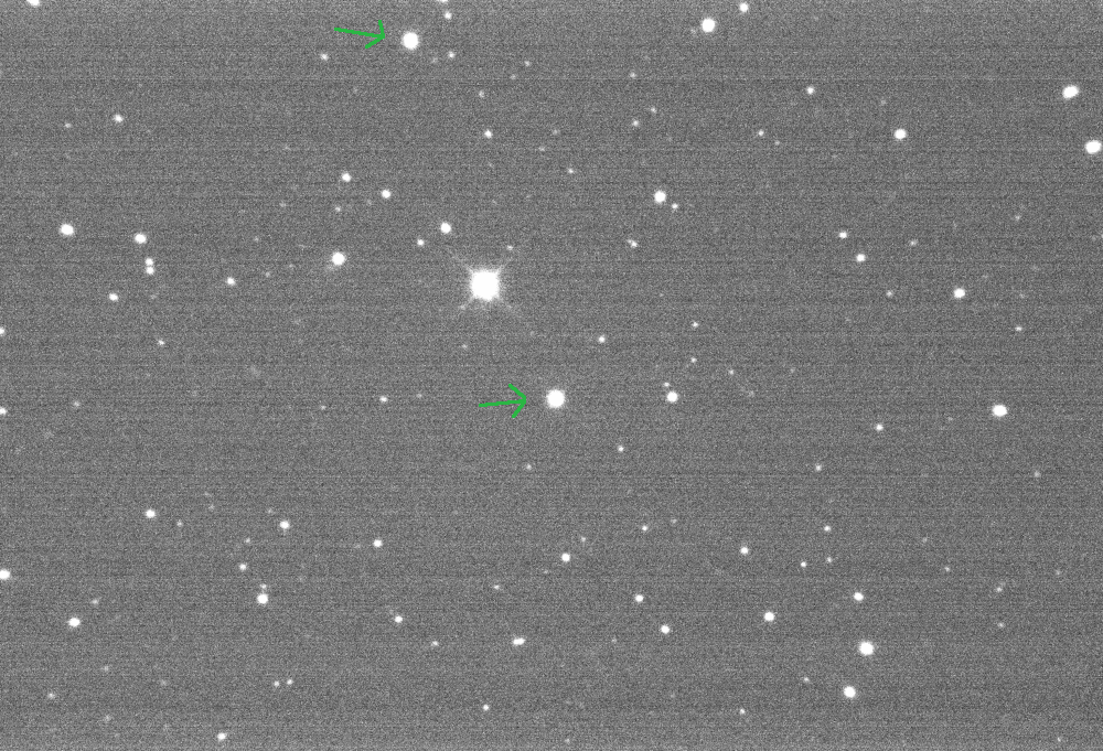
provides both pixel location and sky coordinates of two brighter stars on opposite sides of our target, cou1333. Then astropy SkyCoord.separation computes the angular separation, 211.88567303817118 arcseconds. From the pixel coordinates of the indicated stars, the separation in pixels is 727.43897225043697365183 px. So the telescope + camera with 4x4 binning comes to .2913 arcseconds per pixel, .0728 arcseconds per actual pixel.
Using a diffraction grating
This diffraction grating has period d = 15.17 mm: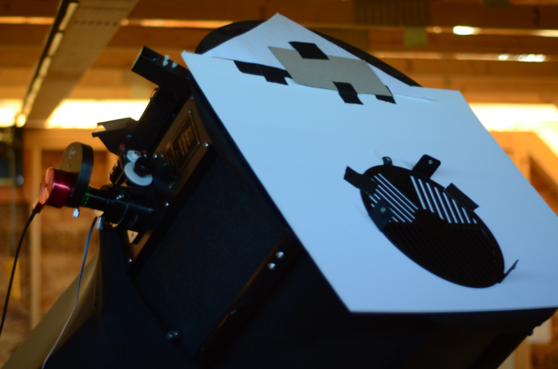
Pointing the telescope at Sirius with this mask and an Hα filter:
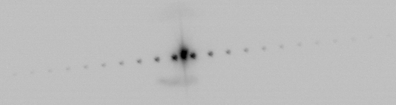
The diffraction grating formula says sin(θ) = λ/d.
With λ=0.00065628 mm, θ = .00004327 radians or 8.925 arcseconds.
The distance of the first spot from the central spot is estimated at 31.14 px, so this route yields 0.2866 arcseconds per pixel, slightly less than the plate solve approach.
cou1333 images
Our goal is to extract a separation measurement (ρ) from 200 exposures.
raw images
Here's one: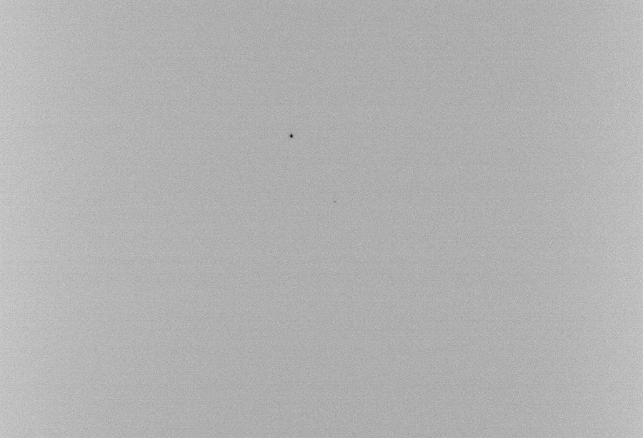
Field of view: 10'x7'. Exposure: 1/100 second.
signal to noise
Zooming in to get a feel for signal to noise (SNR):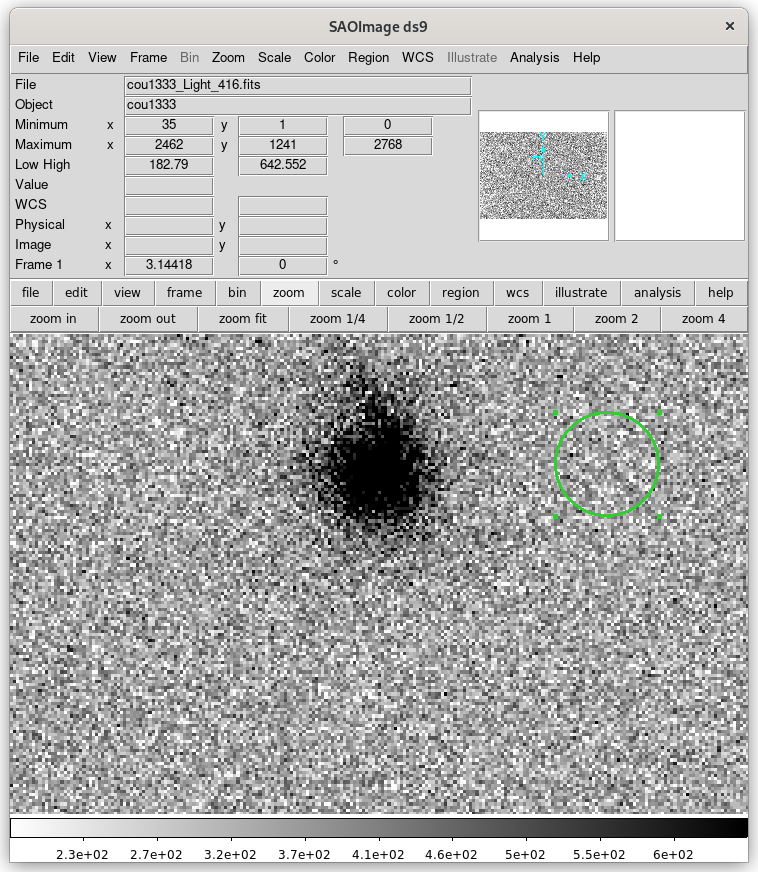
The average intensity in the 862 pixels around cou1333: 778 counts
The average intensity of sky: 339 counts
SNR sample: 2.3
Extracting a region of interest
We average each pixel with its immediate neighbors and extract a 128x128 subframe around the brightest one. Here's the first one: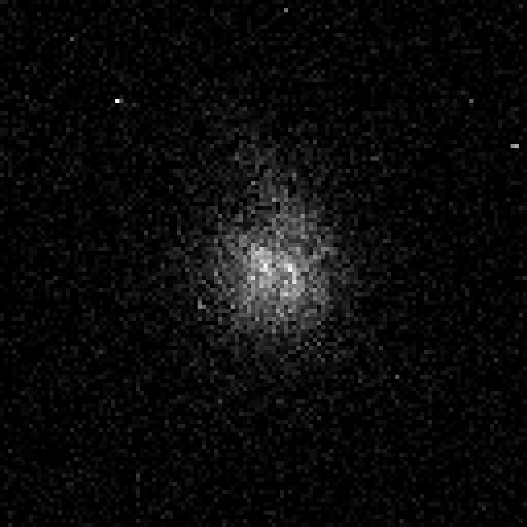
Jumping to SAO ds9 fits image viewer...
Fringes
Following Tokovinin, Mason, Hartkopf "Speckle Interferometry...", 2010, implementation of Labeyrie (as best I can).- Compute the power spectrum of each image
- Compute average of power spectra
- Filter noise
- Divide by best guess at MTF
- Fit model to fringe
Distance from center to peak of fringe ~16 px corresponding to a plane wave with period 128/16=8 pixels.
Using angle subtended by a pixel = .0728 arcseconds, multiply by 8 and get .5824 arcseconds.
posted at: 14:57 | path: | permanent link to this entry
Mon, 12 Dec 2022
Edging Below Half an Arcsecond Double Star Separation
Looking at double star HLD4, discovered in 1881 by E. S. Holden, I got a reasonable estimate of separation (ρ) of 0.48 arcseconds. Besides what appeared to be good viewing on November 17, 2022, it seems it helped to increase the number of exposures from my typical 400 to 800. Since HLD4 is a closely matched relatively bright pair of stars, the speckle diagram was obtained from exposures taken at 0.005 seconds each.
Next, I Turned to a more challenging, dimmer pair, HU1076 discovered by William Hussey in 1904 with magnitudes 10.5 and 12.0. I obtained this specklegram:
I calculated the separation to be 0.53 arseconds, probably 0.09 arseconds wide of the mark. A more accurate measurement might be obtained with more exposures. A more careful look at signal-to-noise ratio may also be in order. It was interesting that a definitive specklegram could only be obtained for a narrow estimate of noise. For in computing the specklegram, I needed to threshold the data at 38 count minimum, this when star pixel maxima might be around 45-49. It was also necessary to threshold no higher than 40 in order to obtain a definitive specklegram.
posted at: 23:53 | path: | permanent link to this entry
Wed, 16 Mar 2022
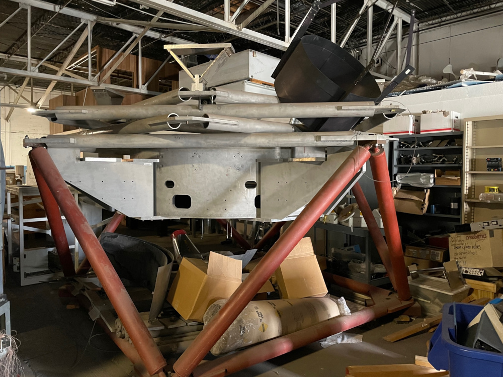
Salvaging Scientific Detritus.
Several mirrors were made during the development of the Hubble Space Telescope. Three full-scale 2.4 meter mirrors were made. One, apparently by Itek corporation, went first to a classified military project and then, when the project was abandoned, to the Magdalena Ridge Observatory in Socorro County, NM. Although operated by New Mexico Tech, it may yet serve military purposes as a fast tracking telescope. And maybe not as there are more modern such scopes that have operated at White Sands Missile Range (Mark Cornell knows about these things). The second mirror, made by Kodak, was never used -- not even aluminized -- and is on display the Smithsonian. This mirror was never used for anything else since it was constructed to be lightweight and, consequently, maintains its proper figure only in zero gravity. The third mirror is the one currently in use on the Hubble.
The company that won the contract to provide the optics for the Hubble, Perkin-Elmer, had first constructed a smaller proof-of-expertise mirror. This is mentioned in the Pullitzer Prize 1991 series by Capers and Lipton. They refer to the prototype as a five-foot mirror. What does one do with such an artifact?
Now, also in New Mexico, in storage in a Physics/Engineering shed on the campus of UNM for the last 9 years is a sort of telescope, something called a transit instrument. In less technical terms, it is a telescope that does not move, so it only observes the objects that rotate into view as the world turns. This instrument came to UNM from Kitt Peak, University of Arizona, in the care of John McGraw, a professor of astronomy who also transferred from UA to UNM. John says the mirror was a Hubble Space Telescope prototype. This mirror is 6 feet in diameter. I suspect it is the Perkin-Elmer mentioned by Capers and Lipton despite the size discrepancy, although it is certainly possible yet another prototype was made.
The main barrier to installing the mirror in a tracking telescope as with the Kodak backup mirror, is that, to save weight, the mirror is constructed as a thin sheet of glass over a lattice support, fine in zero gravity, and fine also when laid flat or nearly so, but not fine when tilted a significant degree. The transit instrument was used at a 4° tilt in its observatory at Kitt Peak.
Jihying and I have committed to building an observatory and resurrecting the instrument on our land near Magdalena if UNM will release it. Perhaps with the aid of local skill it is possible to extend John's technique to support the mirror at angles even greater then 4°.
Salvaging the detritus of big science? Or completely Quixotic? Or both? Hmmm.
posted at: 10:05 | path: | permanent link to this entry
Tue, 15 Mar 2022
Some Observations of Nearby Physical Double Stars
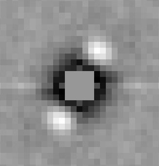
A look at four nearby double star systems, KU39, MLR697, RST5366 and BU1191. These are speckle autocorrelograms derived from series of 400 exposures each taken outside Magdalena Feb 7, 2022.
KU39
KU39 is 57 ly away. KU39 is a closely matched pair with 10.4 mag primary and 10.7 mag secondary (visual light, Gaia BP passband, ~300-700 nm). Orbital elements have been computed for this pair, according to which the angular separation between the two elements should be .61 arcseconds. Gaia EDR3, however, finds the separation to be 1.19". Our own observation put the separation in the neighborhood of 1.13". The last observed entry in the WDS is 1.2", so one doubts the calculation of the orbit.
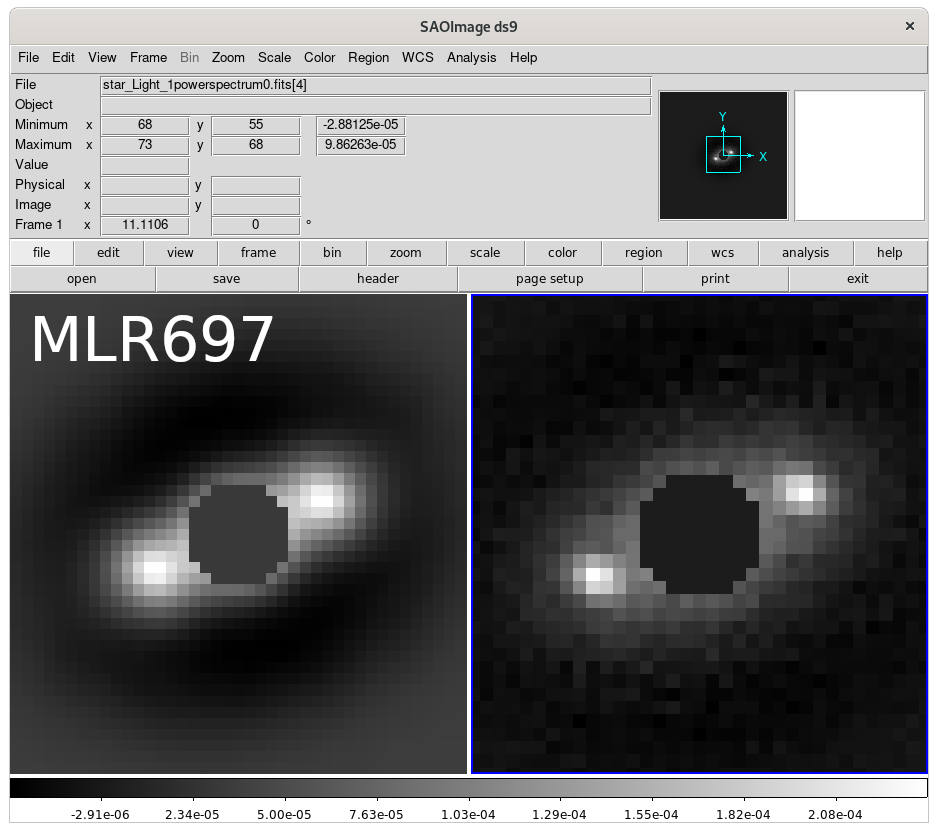
MLR697
MLR697 is 109 ly away and is a very closely matched pair with 9.9 mag primary and 10.0 mag secondary. In contrast to KU39 this pair does not have a calculated orbit. In fact there is only one observation recorded in the WDS catalog dating 1989 with separation 0.5". Gaia EDR3 records separation as .802". Our own measurements depend on the high-pass filter with a low of .759" and a high of .847", averaging .803" on one run to 200 exposures and a low of .757" and a high of .846", averaging .802" on a second run of 200 exposures. The jumps in our calulations stem from the difference of brightest pixel in the autocorrelogram as high-pass filter parameters are varied.
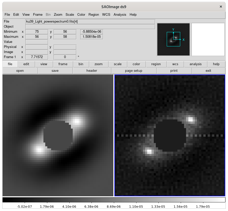
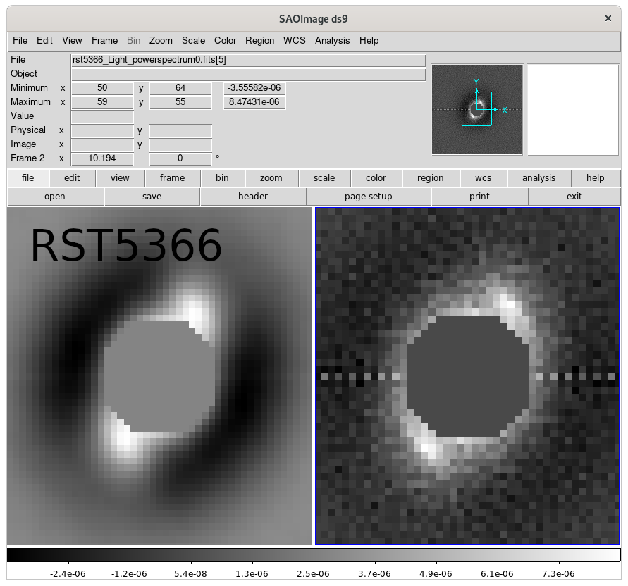
RST5366
RST5366 is also 109 ly away. In this case the secondary component is much dimmer than the primary, its magnitude in visual light listed as 12.7 in the WDS catalog, 2.44 mag dimmer than the primary mag of 10.26. There is no corresponding measurement in the Gaia data releases. However, in the broader green band, ~400-900nm, the magnitude of the secondary is given as 10.8, or 1.4 magnitudes dimmer. Our measurement of separation is clear but not so sharp: 1.11". This is way off both the Gaia and WDS measurents of .88". Perhaps the large magnitude difference corrupts our measurement, but the direction of error is not so clear (see below). If the secondary component magnitude in visual light really is 12.7, the this would extend the limiting magnitude of my 25 inch system with ZWO ASI183MM camera further than I had realized before.
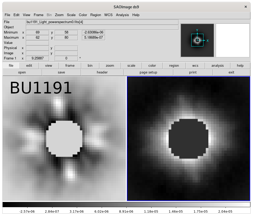
BU1191
BU1191 is the closest of these pairs at 48 ly away, and the magnitude difference is the greatest: 3.9 mag in Gaia's green passband, 4.8 mag in WDS visual light. However, separation listed in Gaia EDR3 (2014-2017) and WDS (2016) agree at 2.0". However, an orbit has been computed for this pair and predicts current separation to be 1.0". I measured the separation to be 1.6". Is this another inaccuracy or did the star move?
posted at: 00:42 | path: | permanent link to this entry
Sun, 24 Oct 2021
Journey to 11th Magnitude
Most of the stars we see in the night sky are large and intrinsically bright while statistically speaking most stars are smaller and less luminous. (See Wikipedia "Stellar classification".) That means stars can be relatively nearby and quite invisible to the naked eye. For example, in the center of these images is a binary star which is "only" 51 light years away and yet a dim 11.42 magnitude in the visual spectrum.
Because the binary system is relatively close, the components are close enough together to complete an orbit in human scale time, 130 years here, and far enough apart to be split visually, components are 1.25 arcseconds apart here. This allows for its orbital elements to be computed with some confidence. (See Stelle Doppie data for WOR11.)
I learned about this double star from data accompanying a paper that analyzed the visual double stars in the Gaia 3rd data release, "A Million Binaries" by El-Badry et al and sent to me by B MacEvoy. I used the 25" Slipstream dob recommended by Bob Pody. The scope is controlled by a Sidereal Technology system which both Dan Gray and Taj Wurl-Koth generously helped adapt to a Linux OS. That enabled the use the Kstars/Ekos/INDI software suite to coordinate the mount, the focuser, the plate solver, and the camera. It is a wonderful open source software project, but I would never have got it going without critical help from Mark Cornell. And finally, if equiment fails, there is no steadier pair of hands around than Eric Toop's or more helpful than John Lebrecque's.
It is no great shakes, of course, to image an 11th magnitude star. The top image is a 1 second exposure at 2083 mm focal length with a ZWO ASI183MM set to 200 gain. The challenge for me was first even to find it and second to image with short exposures, short enough to "freeze" the atmospheric distortion, about 1/50th second, and still have enough signal for, say, speckle analysis. The bottom image is the same field as the first but exposed for 1/50th second.
posted at: 17:56 | path: | permanent link to this entry
Wed, 08 Sep 2021
Wild Pollinators
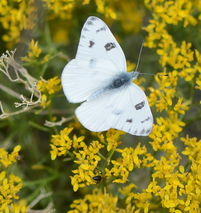
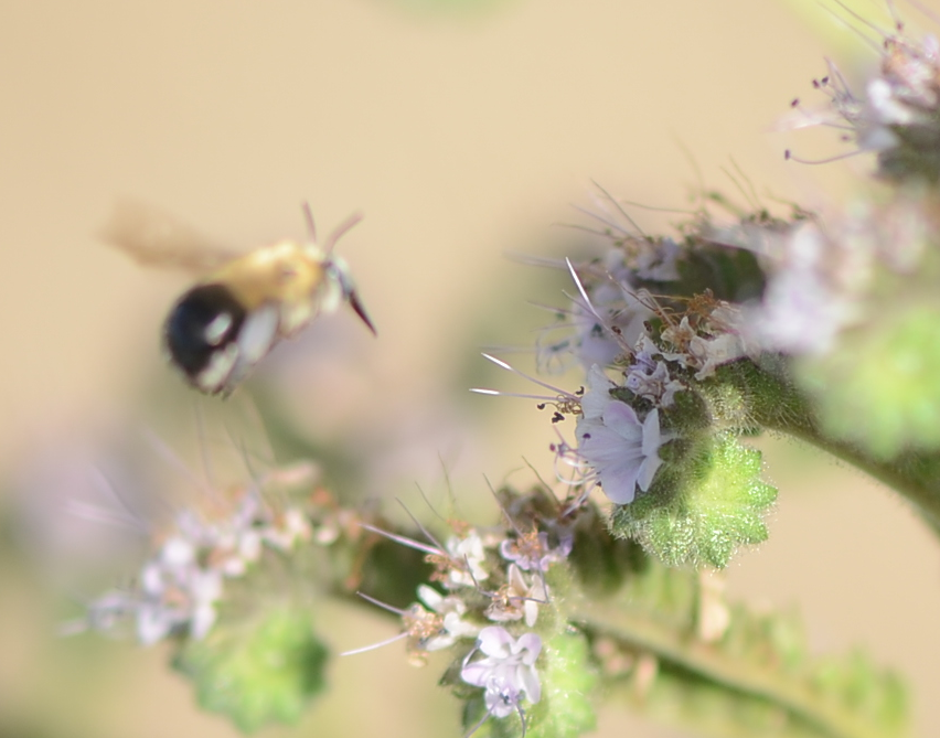
Spring white butterfly and bee visit broom snakeweed out back by the old ranch road ruts. Ranchers don't like the snakeweed because it makes livestock sick, but others have found medicinal uses for it.
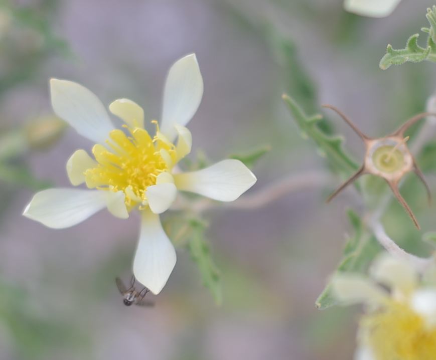
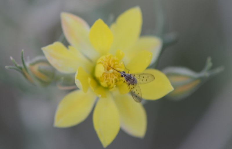
Blazing star wildflower visited by stealth bee-fly near dusk on Camp Lane, Piñon Springs.
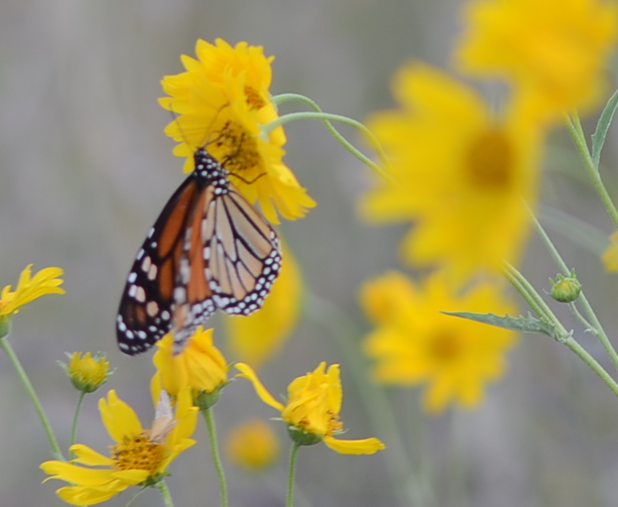
Monarch butterfly on golden crownbeard (cow-pen daisy), near dusk on Campfire Road.
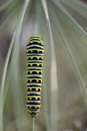
Black swallowtail caterpillar on dill. Jim the EMT in Magdalena gave JY a dill plant which appeared to come with a little something extra.
posted at: 16:40 | path: | permanent link to this entry
Mon, 06 Sep 2021
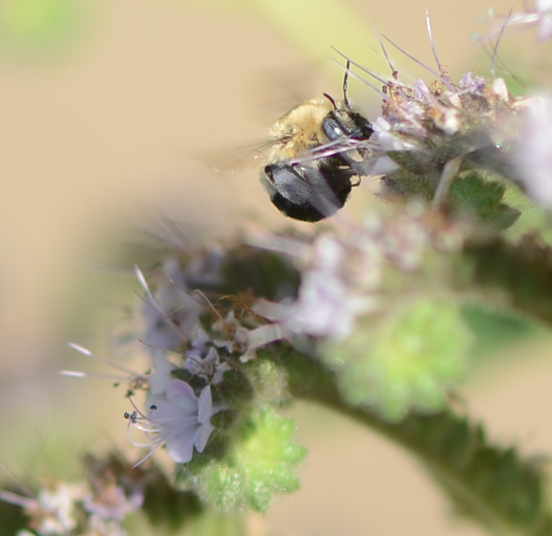
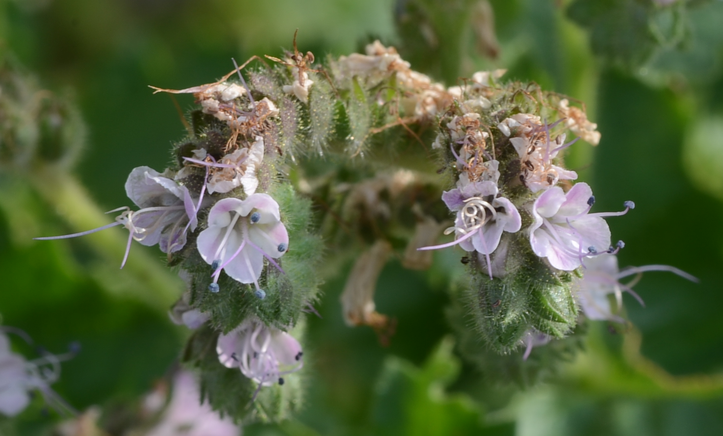
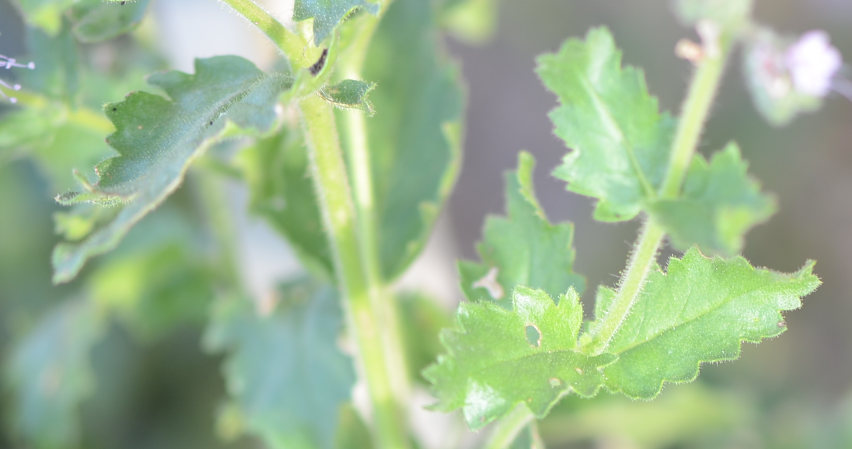
Sivinskis scorpionweed
It's no surprise that most of the wildflowers around our Piñon Springs home have wide ranges, often extending north and south to Canada and Mexico. There is, however, an interesting little plant on the northeast corner of our house that, despite being quite attractive to pollinators, is unique to the Socorro County area, phacelia sivinskii. See documentation at nmrareplants.unm.edu.
posted at: 16:14 | path: | permanent link to this entry
Sun, 05 Sep 2021
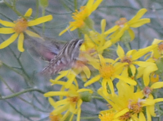
Riddle of the Sphinx
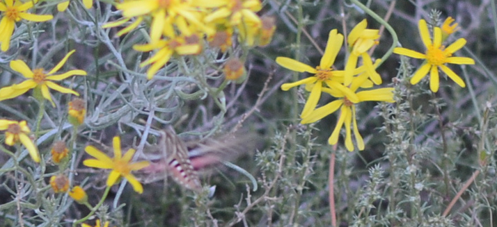
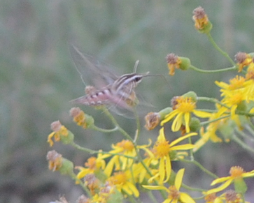
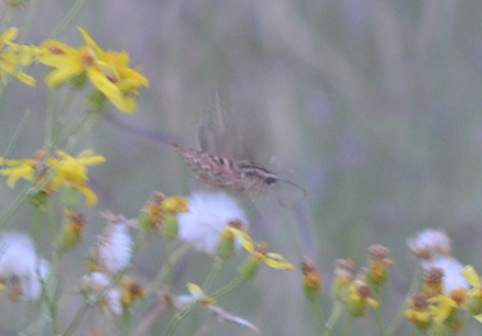
Walking along our Campfire Rd at dusk last week, JY saw something flitting about the damianita bush. It seemed reminiscent of the humming birds we had been seeing during the day; its wing beats even sounded the same; but it was smaller and extremely fast. We tried to capture it on camera. Though little more than a blur, it is clearly the hummingbird moth, the hawk moth, the white-lined sphinx moth. One can even make out its long proboscis.
posted at: 18:24 | path: | permanent link to this entry
Fri, 30 Jul 2021
Importance of a filter for double star measurements
Filters have revolutionized modern amateur astrophotography -- optical filters, that is -- but signal processing filters are of decidedly older vintage. In fact the filter displayed here carries the name of early 19th century mathematician C. F. Gauss. And to apply it, we transform photographic data with a method carrying the name of Gauss's older contemporary, J. Fourier. The revolution in this sphere is the availability to laymen of quality instruments at modest prices.
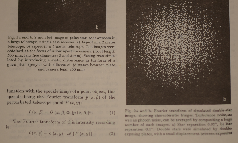
The exercise is to estimate the separation of a close pair of stars, number 2289 in Friedrich Struve's catalog (STF 2289). The method was first laid out by A. Labeyrie in 1970 (Astronomy and Astrophysics, Vol. 6, p. 85 -- available on-line at https://ui.adsabs.harvard.edu/). One starts by acquiring a series of short exposure images. The stars in STF 2289 have magnitudes 6.65 and 7.21. Each exposure was 1/50th second in order to freeze the atmospheric distortion. There are 25 images in this series, 16 of which are displayed in the first attached image. One can surmise there is a multiple star, but measuring the separation appears challenging.
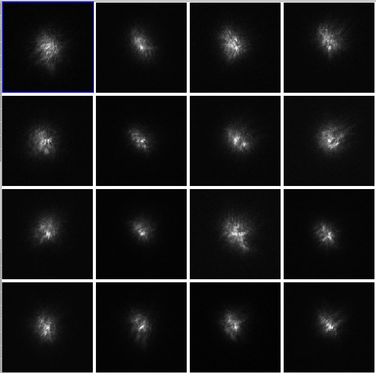
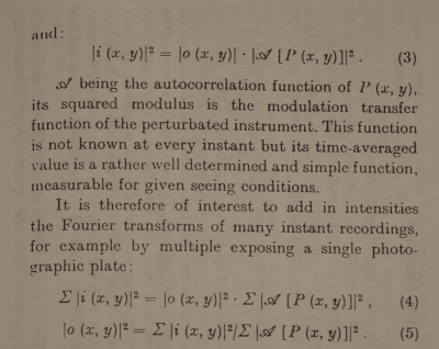
The critical insight is that the atmospheric turbulence manifest in the raw images actually affects light from both stars the same way. And we can see this by taking the Fourier transform of the image data and computing the power spectrum. Adding the spectra together, a spatial periodicity and orientation emerge in the second attached image. One derives an estimate of the separation and position angle but it is still difficult to be precise.
One can compute the inverse Fourier transform of the power spectra to compute the autocorrelation of the image data, but nothing definitive emerges:
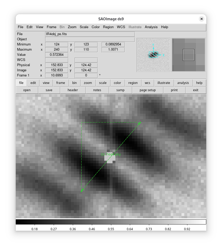
The trick, as explained by Labeyrie, is to filter the data. Here the data is multiplied by a Gaussian function in the frequency domain. In the frequency domain, the filter functions as a mild low pass filter. Viewed in the spatial domain, the image is smoothed, replacing each pixel with a weighted average of pixel values in its immediate neighborhood. With this filter applied, the autocorrelation function does indeed show the presence of double object as illustrated in the fourth image.
Computing the centroid of the secondary maximum, one finds it 12.77 pixels from the center. The images were capured with a 2083 mm focal length telescope, 2.5x "Powermate" Barlow, and 2.4 micron per pixel camera which works out to about 0.095 arcseconds per pixel, and indicates a separation between the stars of 1.21 arcseconds. This is precisely the separation listed for the pair at Stelle Doppie.
This may look better than it actually is. For example, the actual magnification of the Barlow may be a little less. But the moral of the story is how important the right filter is for the application of a fairly modern technicque with very modern equipment.
posted at: 12:09 | path: | permanent link to this entry
Thu, 13 May 2021
Testing my 25" Diameter Slipstream Telescope and ZWO ASI183MM Camera
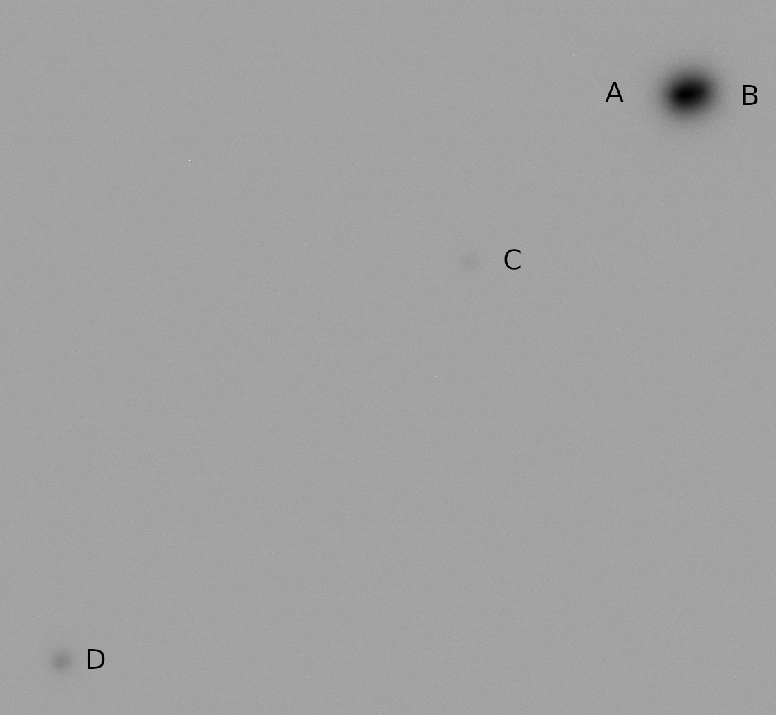
These two images of the star system STF1879 illustrate some properties of telescope and camera used to capture them. Only the two stars A and B are gravitationally bound. Parallax measurements show that A and B are 44 parsecs away while C and D are much further away.
The first image, exposed for 1 second at gain 65 on the ZWO ASI183MM shows the four stars A-D listed for the system in the Washington Double Star catalog. From SIMBAD one can find that the magnitude of star C is greater 13, 13.23 in visual light. Star A is magnitude 7.72, so star A is about 160 times a bright as star C, and the dynamic range of the camera is over 5 magnitudes as the image of A is not saturated.
The second image was exposed for 20 milliseconds at gain 65 and shows the separation of A and B. These two stars are about 75 AU apart -- dwarf planet Eris is about 68 AU from our Sun -- and revolve about each other in about 250 years.
The second image also hints at limits of 20 millisecond exposures with this rig (~0.3 square meters of light gathering mirror effectively focused at 5 meters). At magnitude 13.2 star C is close to the limit of detection with 1 second exposures, so the detection limit for 20 milliseconds should decrease by about 4.2 magnitudes to about magnitude 9. For example, we wouldn't expect to be able to detect star D at magnitude 11.6, and, indeed, we cannot.
posted at: 17:56 | path: | permanent link to this entry
Sun, 04 Apr 2021
Speckle Interferometry
The autocorrelogram provides an intuitive explanation of speckle analysis, but Fourier analysis provides a framework for inverse filtering (deconvolution) as developed by Labeyrie in 1971. Here is a look at a model and an example.
Part 1: Model
The idea starts out the same in both views. Namely the observed image I is the sum of several images, each the diffraction limited image O having passed through a different cell of air with its own refractive index resulting in a shift of O by a random vector u_j. (Following the Teχ convention of using the underscore to indicate a subscript and letting n denote the number of images.)
I = (1/n)Σ_j O * δ_(u_j), j = 1...n
That is, under the assumption of shift invariance and non-distortion, I is the convolution product of the system input image with the point spread function (PSF), the output image of a point source, here expressed as an equally weighted sum of delta functions.
The Fourier transform of I, F(I), is linear,
F(I) = (1/n)Σ_j F( O * δ_(u_j))
and the transform of a convolution product is the point product of the transforms,
F(I) = (1/n)F(O) ∙ Σ_j F( δ_(u_j))
and the transform of the delta function is the plane wave,
v → exp( -i ∙ v • u_j), v ∈ ℝxℝ
where the bold dot (•) indicates the vector inner product. So taking just the modulus squared of the Fourier transform,
|F(I)|²(v) = (1/n)²|F(O)|²Σ_(j,k) exp(-i · v • (u_j - u_k)), j,k = 1...n,
the product of the transformed input image with the modulation transfer function (MTF). When j = k, the summand equals 1. For the n(n-1) summands where j ≠ k, a real-valued interference term is obtained, cos(v • (u_j - u_k)). If the u_j are independent normal random vectors with variance σ², then the expected value of cos(...) is exp(-|v|²σ²).
If numerous images are captured and the distributions remain stationary, then the images may be averaged. Then, assuming v constrained by the frequency limit of the telescope, by the law of large numbers,
<|F(I)|²(v)> ≈ |F(O)|²(1/n + ((n-1)/(2n))exp(-|v|²σ²))
as the number of samples increases.
Special cases. If n = 1, then the MTF is simply 1, of course. For n > 1, the MTF is a sum of a constant and a Gaussian. If n = 2, then the MTF is
1/2 + exp(-|v|²σ²)/4
And if n = 3, then the MTF is
1/3 + exp(-|v|²σ²)/3
As n increases, that is, the more refracting cells and choppy the air, the balance shifts from the constant to the exponential. As σ² increases, the variance of the Gaussian, proportional to the reciprocal of σ², decreases. Both have the effect of bunching the system response into lower frequencies and suppressing the higher, hence limiting angular resolution.
If O were simply a point source, then looking in the space domain, it's autocorrelation, ideally a single point, would be partially obscured by interference among the speckles, represented here as linear combination of δ₀ and a Gaussian with mean 0 and variance now proportional to σ².
Now suppose that image O is the sum of two point sources, like a double star, say one point at the origin and the other at point w, δ_0 and δ_w with Fourier transforms constant 1 and plane wave v → exp(-2πiv•w). The power spectral density is then
2 + exp(-2πiv•w) + exp(2πiv•w) = 2 + 2cos(2πv•w)
which when transformed back to autocorrelation becomes the triple sum of delta functions
2δ_0 + δ_w + δ_(-w)
Thus, in the presence of speckle noise, we have in the frequency domain
v → (2 + 2cos(2πv•w))(1/n + ((n-1)/(2n))exp(-|v|²σ²))
and taking the inverse transfrom, one recovers the two star autocorrelation with Gaussian noise added in, possibly enough to obscure the relative maxima of the autocorrelation. Of course, if this PSF were a good guide to actual observation, one could use the MDF to construct an inverse filter.
Labeyrie's approach to the PSF was suggested by star photographs and Kolmogorov's model for atmospheric turbulence. Starting there, astronomers have developed more sophisticated models. For example, Jack Drummond has developed a model of the PSF as a sum of a Bessel function and the Cauchy distribution. (Thanks to R. Q. Fugate for the reference).
Part 2: Example of inverse filtering, STF 848
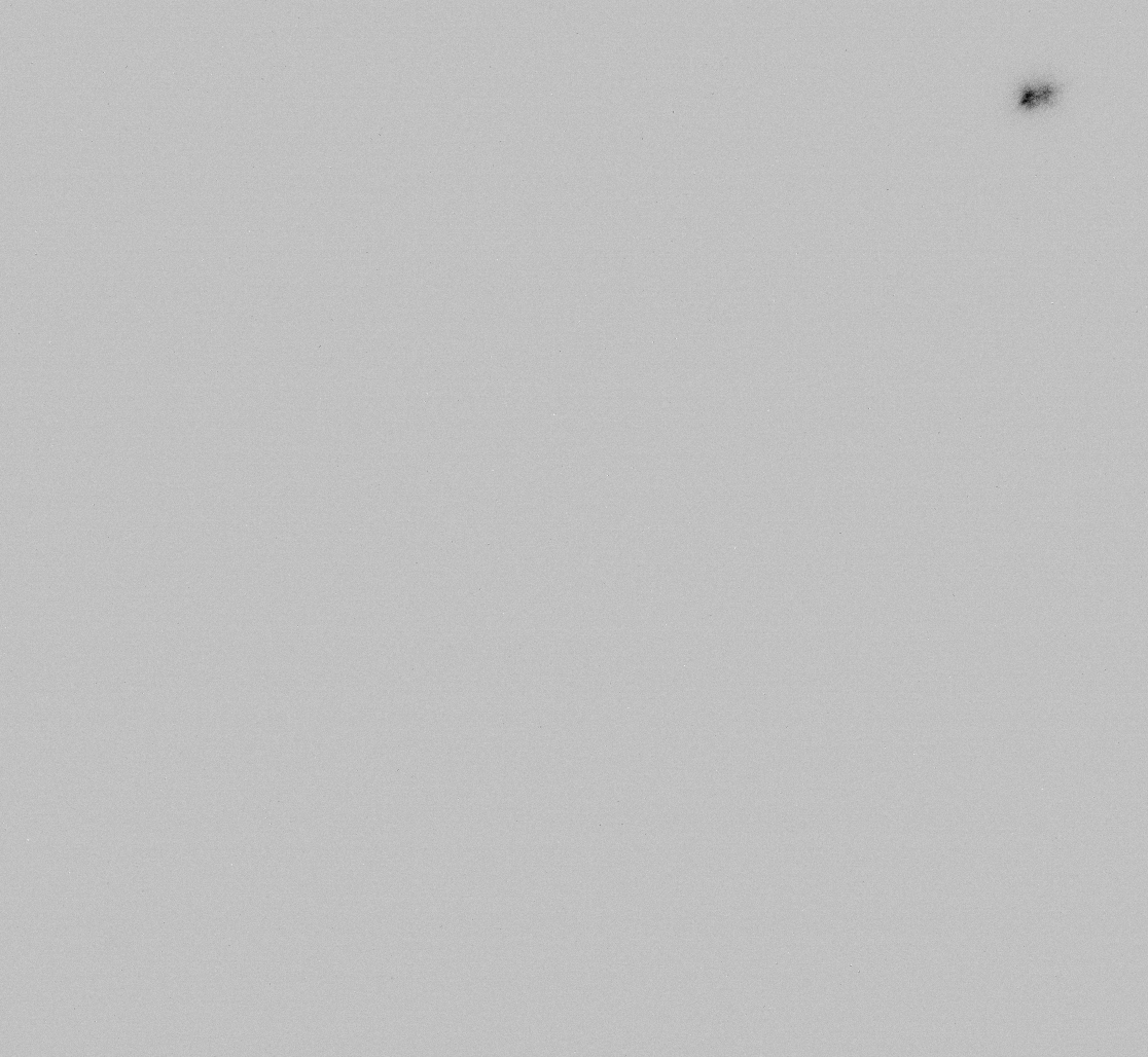
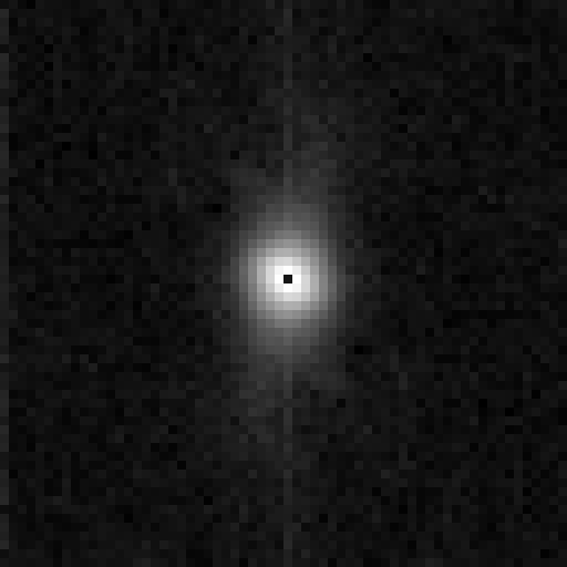
Data: 25 images of double star STF848 (Henry Draper 41943), each exposed for 5 milliseconds each. Here is an animated GIF of the first fifteen (refresh to run again):
We take these images and compute their autocorrelatograms and average them together, essentially checking to see whether the triple of delta functions above can be distinguished through the noise:
Suggestive perhaps but actually nothing pops out; there is only one local maximum.
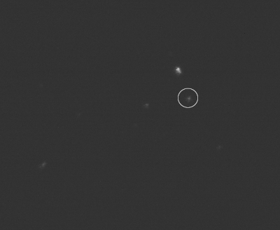
So, following Labeyrie, we try an inverse filter, one where the filter divisor is obtained by approximating the PSF. The double star STF 848 sits in the "37" open cluster in Orion, and our images contain additional stars in the same frame. In particular STF 848 itself is assigned a visual companions. STF 848D, magnitude 8.3, is circled here in the first frame of our set; STF 848 A and B comprise the bright blob above it:
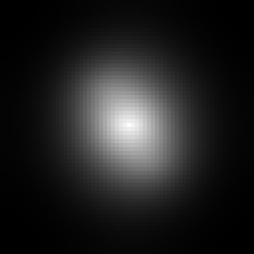
Using the 25 exposures to compile an average MTF for STF 848D, we construct the unassuming composite:
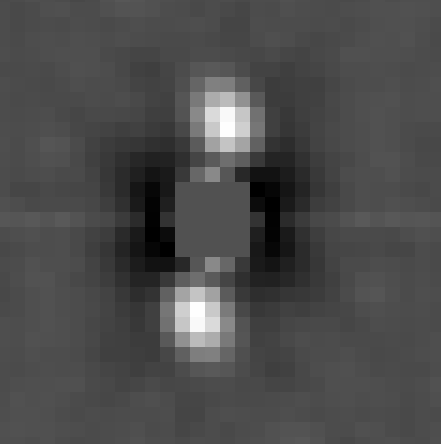
However, when we compute the element-wise quotient of the average STF 848AB MTF by the average STF 848D MTF and then take the inverse Fourier transform back to the spacial domain to obtain the filtered autocorrelogram, we get this:
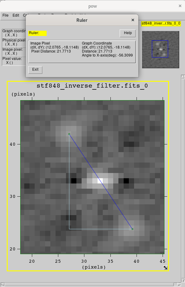
where suddenly the triple peaks of a double star autocorrelogram can be detected.
Using the ruler tool in the fv FITS viewer for instance, the side peaks are found to be about 21.77 pixels apart. The instrument used here has a focal length of 82 inches and the camera has 2.4 μm wide pixels, hence about .238 arcseconds per pixel. Thus 21.77 px translates to 2.587" separation between STF 848 A and B stars. The "precise separation" listed at Stelle Doppie is 2.605" for agreement within .1" with our estimate.
Scientists have developed many filtering techniques including blind deconvolution using the model above and Gaussian speckle-masking described by A. W. Lohman et al, 1983, (thanks to D. Elmore for introduction to speckle masking) when no reference star is available.
posted at: 11:58 | path: | permanent link to this entry
Wed, 24 Mar 2021
Telescope Builder
On March 6th JY and I hitched up the Jayco toy hauler to our pickup and took off for California. It was our first trip back to California since we had left Irvine, small U-Haul in tow and JY pregnant, August 1983.
From Magdalena we headed west on US 60 past the VLA, Pie Town and Quemado, then northwest skirting Petrified Forest National Park and west on I-40 to the Las Vegas turn-off where we rested for the night.
Sunday morning we drove north, first by the beautiful Lake Meade National Recreation Area, then through the vast expanse of sin city and onward through an breathtaking panoply of mountain ranges along the eastern flank of the Sierra Nevadas, skirting Death Valley and then Walker Lake and the eerie metropolis of ordinance mounds just south. Arriving in Reno, we camped for the night and left for Grass Valley through snow flurries in Donner Pass.
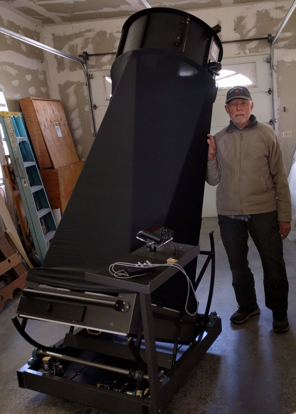
There we met Tom Osypowski living with his wife in quiet seclusion at the end of a narrow gravel lane outside the old gold rush town. Inside his machine shop, a gleaming new Dobsonian telescope awaited us.
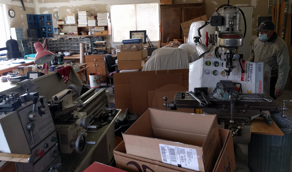
Asked how he came to astronomy and telescope making and about a beautiful lunar astrophotograph, Tom had this to say:
My astronomy adventure started when I was about 12 years old. It was like some kind of urge just turned on and told me to look at the night sky. I soon got a star atlas and learned the constellations and the names of the stars. Soon after I wanted to get a telescope to look at the planets. It quickly mushroomed from there and before long I was building my own telescopes from surplus parts. This was back in the mid-50's. I joined a local astronomy club, the Milwaukee Astronomical Society. They had an observatory out of town and I spent as much time as I could there using the 13" reflector mounted in a dome. It was with that telescope that I took the picture of Plato and the Alpine Mt range that you saw in my shop. I stayed with my astronomy proclivities until about '65 and then took a sort of sabbatical from that pursuit for 17 years until I moved to the area in CA I now live in. The dark skies here, and another of those "urges" had me building telescopes again and observing the night sky. In 1982 the Dobsonian revolution took hold and I had soon built a 16" dob that won some awards at RTMC. A year later it was equipped with my first Equatorial Platform, a device that was just beginning to take hold of the dob world. The Platform was a huge success and friends asked me to build one for them too. Soon I had a business that I am still working at, 35 years later. Since that first Platform, I have built about 700 more of them for customers. I also started offering complete metal telescopes about 22 years ago, and have built dozens since then. Yours is the latest, #42.
He also reminisced a little about the old days of film photography, dark rooms and enlargers. In passing he also mentioned having lived in Taos a spell, so I asked him for details, and this was his reply:
My time in the Taos area was during my 17 year haitus from astronomy. I was pretty much a hitchhiking vagabond (hippie) for many years, staying in various places, a lot of times alone like a hermit. In New Mexico I had a tiny adobe hut that I lived in. It was in a small town called Arroyo Hondo, outside of Taos. I would walk down a winding trail to the Rio Grande River Canyon that was close by and spend some time in hot springs that were situated right by the river. Also grew a lot of my own food in a great garden I tended. Standing in that garden I could see the snow capped peaks of the southern Rocky Mts. The Sangre de Christo, those peaks were called. The snow off them flowed down in carefully tended ditches to bring water to the towns nearby, and even via a local ditch to the very garden I stood in.
Having packed the new scope securely, we headed west to Sacramento and south through the Central Valley, California's agricultural heartland, then east through the Mojave and back to Magdalena where we rolled the prize into our new observatory.
posted at: 09:14 | path: | permanent link to this entry
Sun, 15 Nov 2020
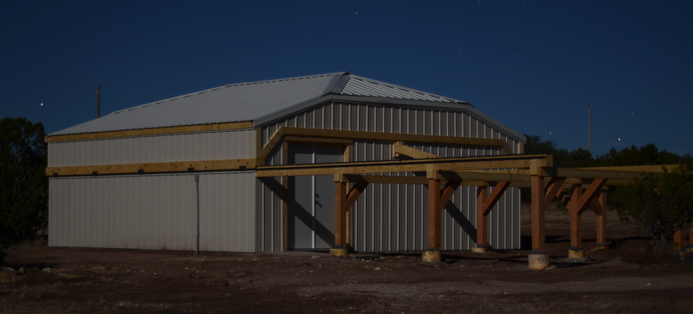
Building an Observatory
Starting just after autumnal equinox this year and finishing just before the October blue moon, we built an astronomical observatory at our home northwest of Magdalena, NM. Our observatory was modeled on the "dobservatory" Backyard Observatories built for the Montana Learning Center. With workforce depleted by COVID, Scott and Diane comprised the entire BYO crew, and just the two of them assembled the 24' x 24' structure in less than two weeks time on a concrete slab poured by True Blue Construction of Magdalena.
Here are a few photos and comments to document the project.
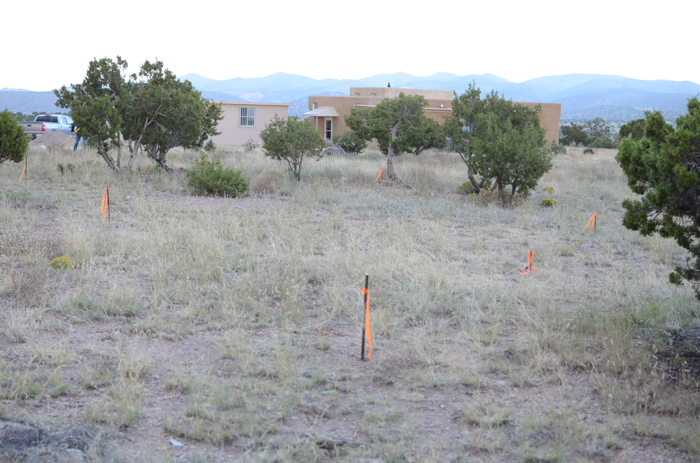
We picked out a spot with a good southern horizon along the ridge that divides the La Jencia Creek basin from the Rio Salado, an easy walk from the house but far enough to avoid disruptive air currents. That's Jih-Ying behind the Juniper clearing away a few tumbleweeds. Those are the Bear Mountains behind the house with an abandoned uranium mine in view just above the workshop window.
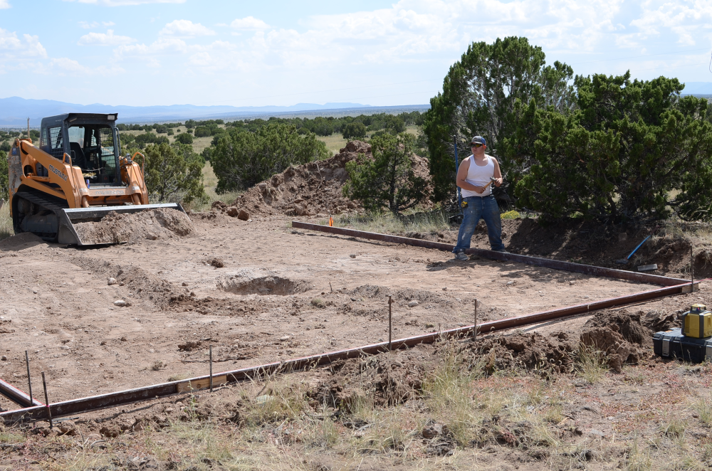
Tyler and his helper, Paul (pictured), leveled the ground, dug a hole for the telescope footing, and set up forms for the concrete slab.
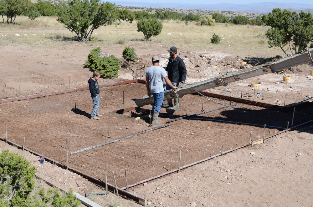
Forms ready, Tyler, his son Cash, and Tyler's concrete guy start the pour with the telescope footing, 3 feet deep and isolated from the rest of the slab to prevent vibrations in the slab from shaking the telescope.

While concrete guy trowels the wet concrete, busy Cash zipping here and there gets caught in the wire mesh and takes a tumble. Unflappable Tyler patiently keeps Cash out of trouble and Cash, out of school, learns a bit about the trade.
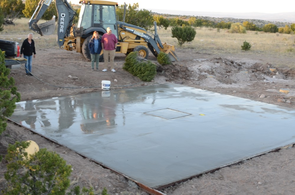
After the concrete was poured, it needed to cure; that is, we needed to keep it moist for a couple days. Water is precious and we don't have a well yet. So John Briggs generously supplied us with a tank of water to use from his well. Jih-Ying, Lori and Mark look on. (John introduced us to Mark and BYO, and Mark found the "dobservatory" on Cloudy Nights. Tyler's new backhoe also posed.
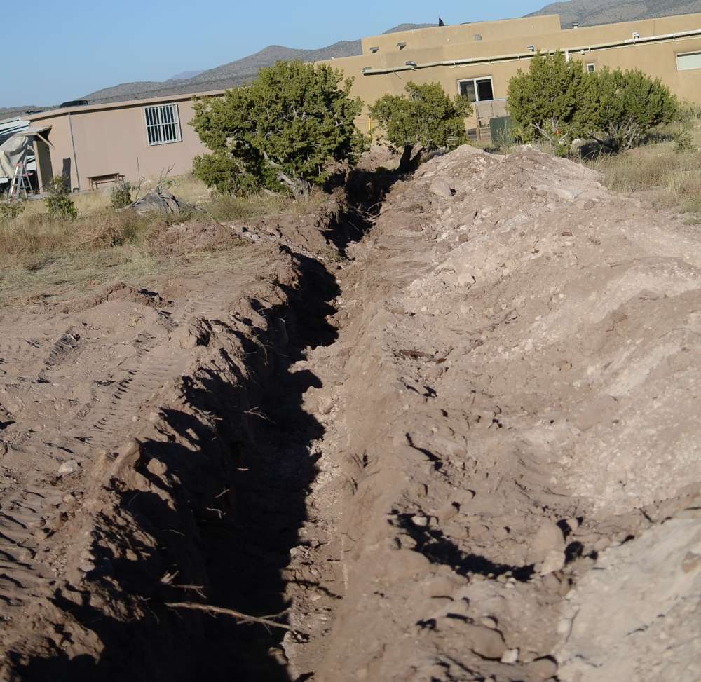
Tyler used his new backhoe to dig a trench so Danny and Barbara Sandoval could run electricity to the observatory.
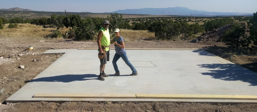
Scott and Diane rolled in Friday night, October 16, big black Mercedes van pulling their COVID bubble travel trailer. They had lumber and siding delivered ahead of their arrival and we able to get started the next morning.
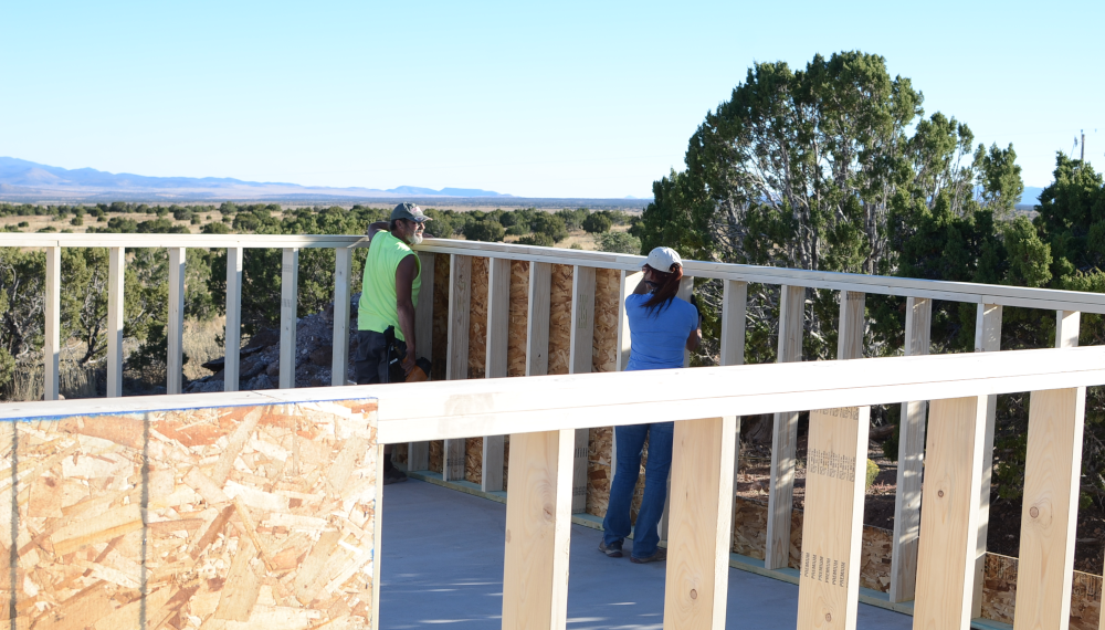
The five foot supporting walls go up first.
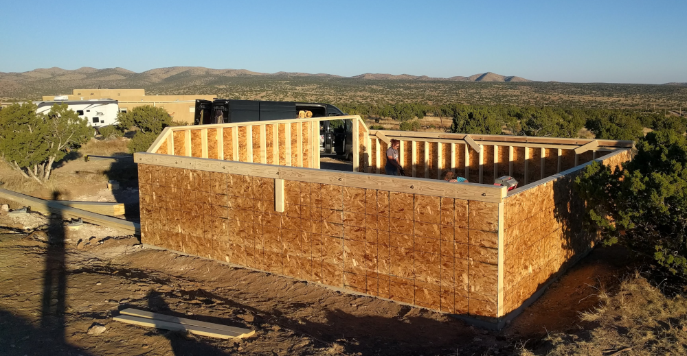
Working past sundown, walls are up and sheathing nailed on. Base for the roll-off roof positioned on rails (note extension to the left) and tacked down to keep from rolling off prematurely!
Scott and Diane, working just the two of them, installed and spaced the trusses with no more tools than a "Y" made from scrap 2x4's: inverting, lifting one end at a time and flipping. Cool.
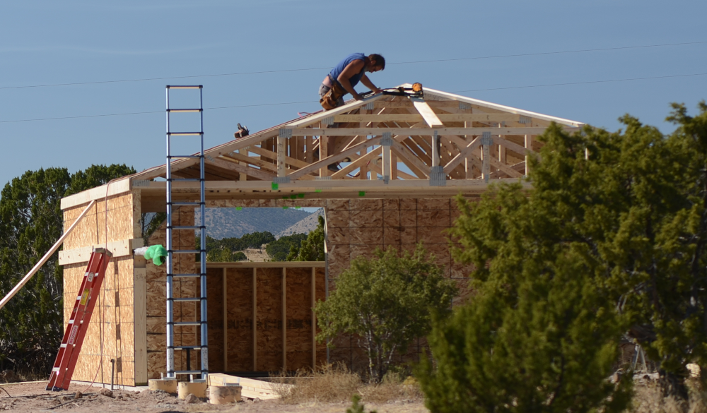
Scott and Diane formerly built houses. In order to give the observatory an extra degree or two horizon in the direction of the door wall, Scott came up with the idea of a partially hipped roof. "Partial" because the ends of the roof still need to span 24 feet without support from the walls.
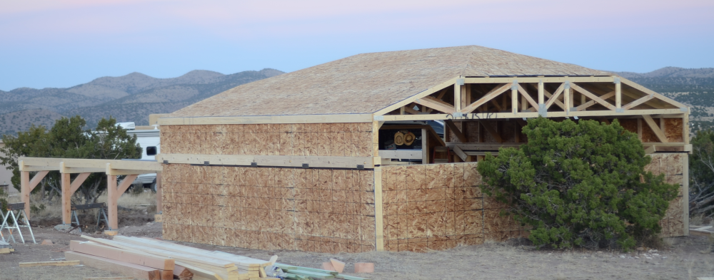
Gantry up. Roof sheathing installed. The upper two feet of the side walls are part of the roll-off roof structure providing extra horizon to scopes mounted on a low axis and head room for humans at the same time. Sort of a hybrid between traditional roll-off roof and a roll-off building like Deep Sky West in Rowe. Opposite the door wall, facing roughly southwest, the upper two feet of wall fold inward.
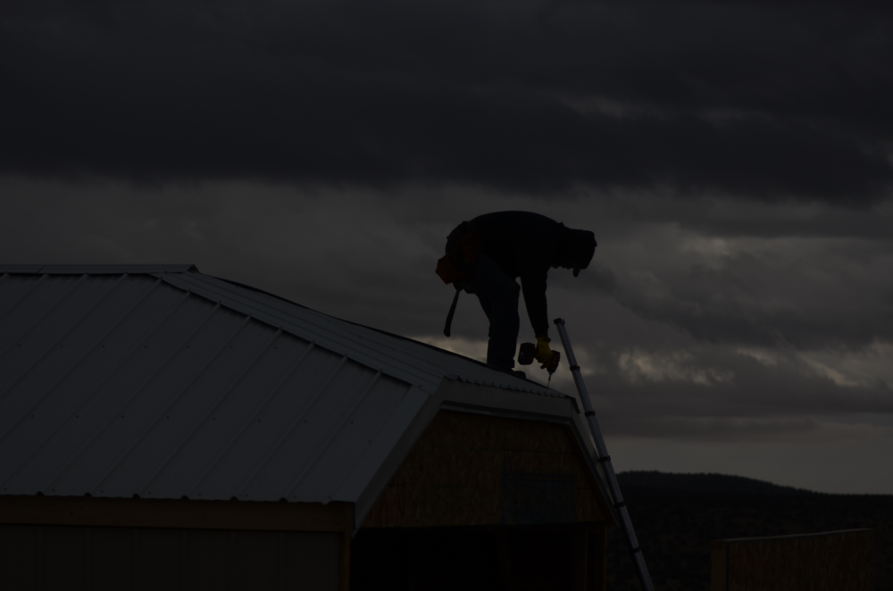
After applying a moisture barrier--sort of a synthetic tar paper--Scott applies a metal roof.
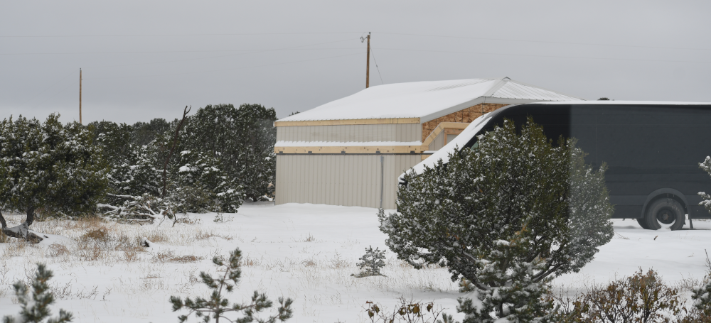
Just hours from completion, an early winter storm blew in. Much needed day of rest for the BYO crew.
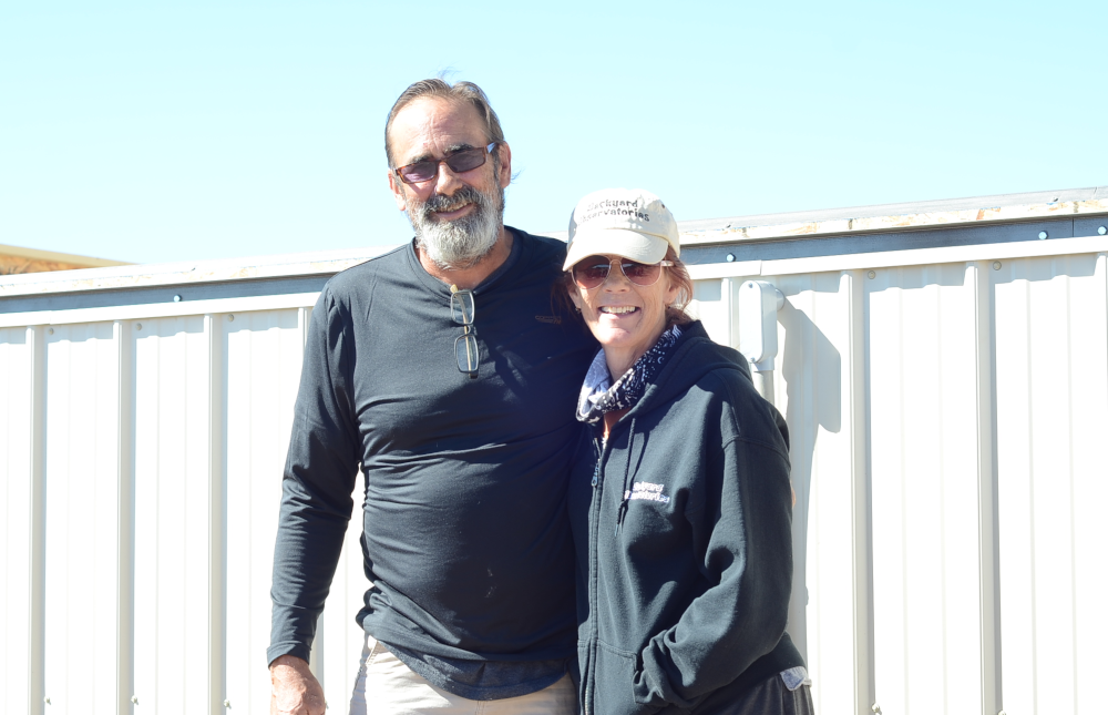
Sunshine returns, BYO finishes up, Scott and Diane head for their next job in Florida with a stop by Ohio to check up on family and pets.
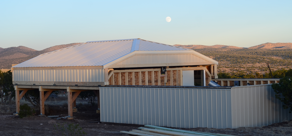
Evening, first day. It works!
Under the stars and full moon.
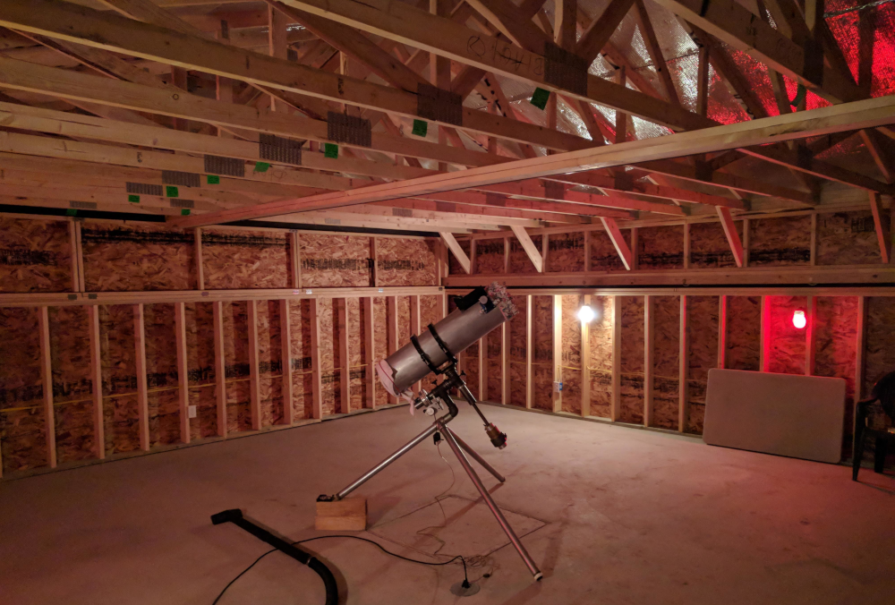
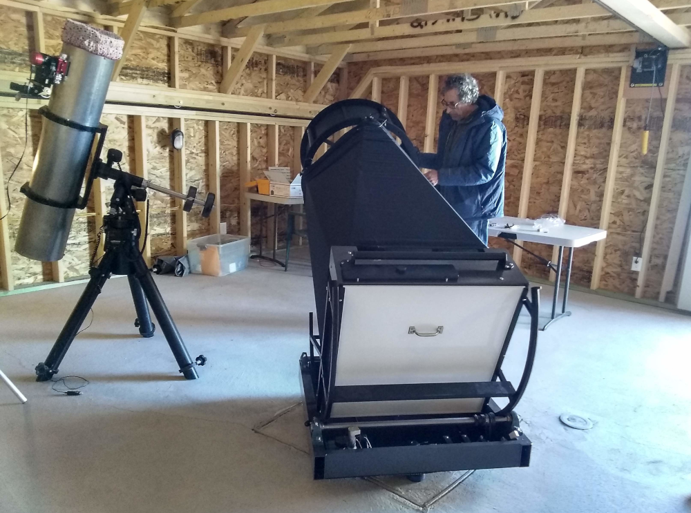
Inside the finished observatory. Wired separately for red and white light. Thanks to Mark's suggestions, power on the floor near the pier footing, radiant barrier on the roof underside. Fold-down wall is visible as well.
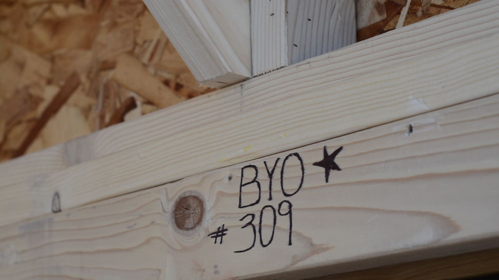
Signed and sealed. Backyard Observatories number 309. October 29, 2020.
posted at: 15:56 | path: | permanent link to this entry
Fri, 13 Nov 2020
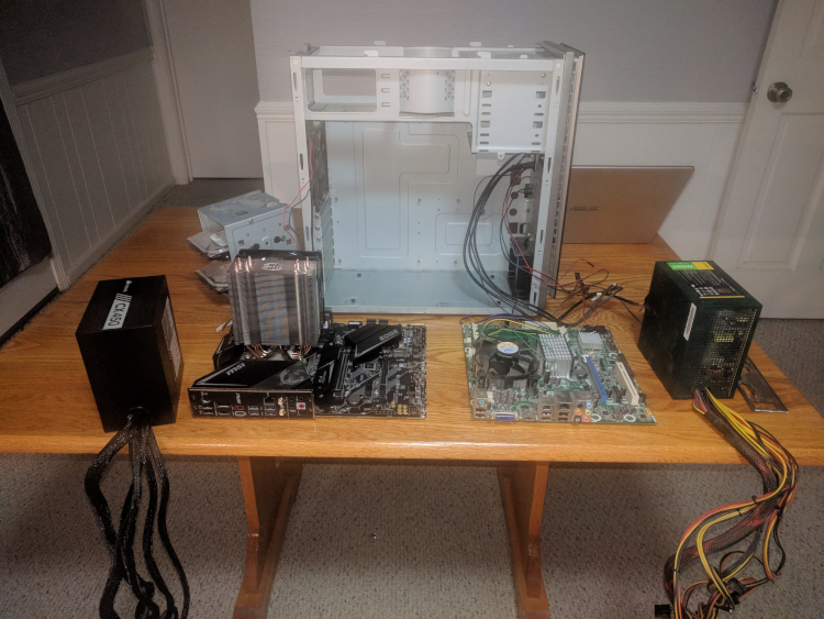
Tod und Verklärung
After about ten years, it appeared that the motherboard of my desktop computer had died. The case and SATA drives and monitor were salvaged but a new CPU and memory were installed on an MSI Z490 "Gaming Edge" board, along with a new power supply and a cool new 1 terrabyte solid state drive the size of a stick of gum. What a difference a decade has made! 16 gigabytes of memory and 6 cores, 4.1 ghz clock.
posted at: 18:24 | path: | permanent link to this entry
Sun, 14 Jun 2020
A Moderately Close Double Star and Seeing Measurements
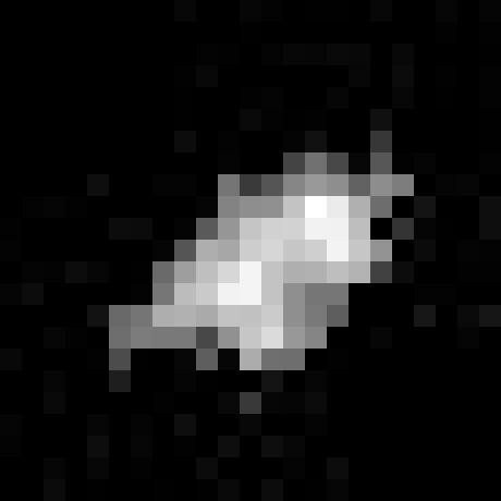
This is a look at double star STF 1757 (F. Wilhelm von Struve) located just a shade north of zeta Virgo, a 7.8/8.8 magnitude solar type binary with K giant according to MacEvoy and Tirion's "Double Star Atlas". I was unable to verify by plate solving at Astrometry.net, but the two nearby stars in the image match up with the C and D stars, magnitudes 11.9 and 12.5, listed in the Washington Double Star Catalog (WDS). This image was captured near midnight May 17th with a ZWO ASI290MM on an 8" f/6 reflector.
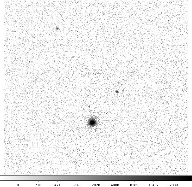
C and D are not physically related to the AB pair although an orbit has been computed for the AB pair, a 461 year revolution at a separation of 73 astronomical units. The WDS also lists the apparent separation as 1.7 arcseconds as of 2018.
Here are two close-ups in SAO DS9 of STF 1757 A and B stars. The first maps file brightness values linearly onto display values while the second uses a convex transformation increasing the visibility of intermediate values.

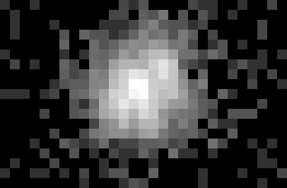
The pixel squares are .49 arcseconds on edge.
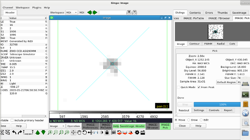
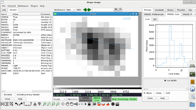
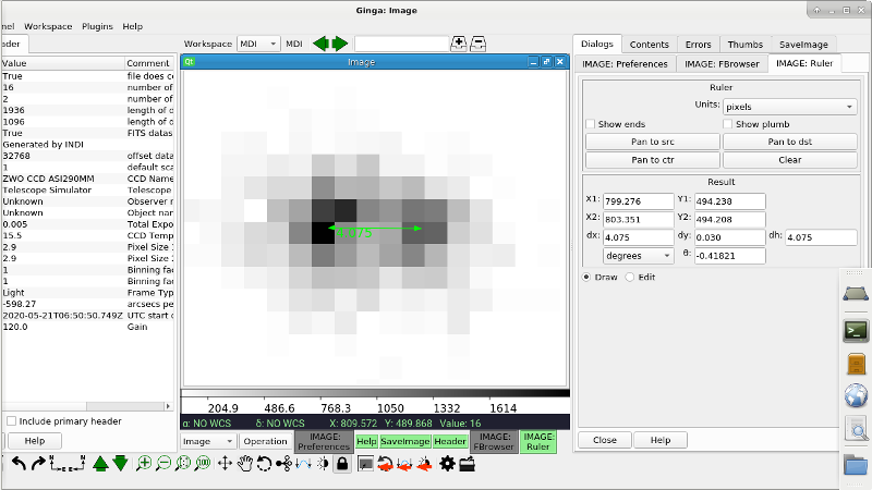
Here is a screenshot from a Ginga (Japanese for "galaxy") analysis of the same exposure. The cut through the two bright areas shows a clear diminution of intensity, hence we may say the image successfully split the double star components. The ruler between the approximate centers of the bright areas reads a distance of 3.54 pixels, or about 1.7 arcseconds in agreement with WDS.
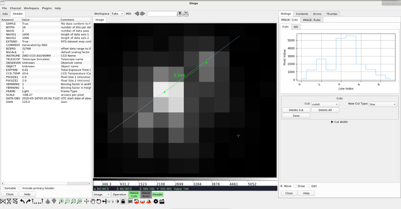
Ideally this would mean that seeing, as measured by "full width half maximum" was no more than 1.7" that evening, and that might actually have been the case during the .01 second exposure. But not all the images were this clear, due either to worse seeing or to telescope shake in the strong breeze.
Working at the scope, I was unable to see that my images were achieving sufficient detail to split the star and on subsequent evenings that week, tested only stars with greater than 2 arcseconds separation.
posted at: 00:57 | path: | permanent link to this entry
Wed, 10 Jun 2020
Using plate solver as a star hopping check
The evening of May 18 I was trying to split a double star as a sanity check on seeing measurements I was taking. Canadian weather had predicted poor seeing (https://weather.gc.ca/astro/seeing_e.html) despite the clear skies. From this and the constraints of my equipment I decided to look for a pair separated by about 2 arcseconds. Hercules was high in the sky and double star Struve 2052, near the front knee, is an evenly matched double with 2.3 arcseconds of separation. Gear was an 8" equatorially mounted push-to Newtonian telescope with a ZWO ASI camera which meant that I needed to star hop over. STF 2052 is relatively faint a 7.7 magnitude so it was a challenge for a beginner like me.
I found my way to Gamma Hercules and thought (mistakenly) I had found the double but was unable to split the pair. I chalked it up to seeing conditions, but as a precaution captured a 1 second exposure, long enough to provide a plate solver sufficiently many stars to determine location. The next morning I uploaded the image to the amazingly nice Astrometry.net. Luckily the solution came back quickly, but, unfortunately, it was difficult to read the annotation since both Tycho and Draper identifiers were written in the same place:
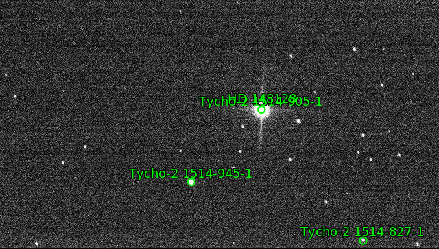
Luckily, Astrometry.net also provides data in text format as well (cf. http://astrometry.net/doc/net/api.html). In my case the XML snippet of annotations looked like this:
{"annotations": [{"type": "HIP", "names": [""], "pixelx": 1153.8204358390917, "pixely": 484.50643604007297, "radius": 0.0},
                 {"type": "HIP", "names": [""], "pixelx": 455.0254442348971, "pixely": 842.2364142131472, "radius": 0.0},
                 {"type": "tycho2", "names": ["Tycho-2 1514-945-1"], "pixelx": 844.7352480090982, "pixely": 803.0079527404176, "radius": 0.0},
                 {"type": "tycho2", "names": ["Tycho-2 1514-905-1"], "pixelx": 1153.8444483449232, "pixely": 484.5007752543975, "radius": 0.0},
                 {"type": "tycho2", "names": ["Tycho-2 1514-827-1"], "pixelx": 1601.7812911350134, "pixely": 1060.7429318451464, "radius": 0.0},
                 {"type": "hd", "names": ["HD 148128"], "pixelx": 1153.844500937562, "pixely": 484.50072816016404, "radius": 0.0}]}
Actually, there was an even more direct approach available. Once Astrometry.net succeeds in solving an image, it regenerates the image into a new FITS file and adds the WCS coordinates of each pixel to the FITS header. Using this information, one may view the image in a FITS viewer and see the right ascension and declination of the pixel underneath the mouse pointer.
The next night, May 19, under similar skies I was better able to match the star chart to what I was seeing in the finder scope and split the double star--at least in the sense of distinct separate bright spots. In this photo, pixels subtend just under .5 arcseconds along the edge, .7 along the diagonal. A little over 3 diagonal distance between bright spots corresonds to an angular separation of 2.3 arcseconds, and the diminution of intensity between the bright spots verifies that seeing was no worse than 2.3 arcseconds.
Using my home-baked differential image motion monitor (Sarazin & Roddier, Bally et al), seeing was in the neighborhood of 1.72 full width half maximum in the same location at about the same time.
Many thanks to Mark Cornell for suggesting this comparison.
posted at: 10:16 | path: | permanent link to this entry
Mon, 01 Jun 2020
Double Stars and Seeing
For the last few trips to our Magdalena home, I've been trying to take seeing measurements as part of evaluation of possible sites for an observatory. A friend who is also a professional astronomer suggested checking whether is was possible to split double stars whose angular separation was near the seeing limit.
One pair, in Coma Berenices, is STT (Otto Struve) 266. From the Washington Double Star catalog the stars are nearly equally bright at magnitudes of 7.97 and 8.42 and are separated by 2.00 arcseconds as of 2018.
It was windy and seeing had been predicted to be below average by the Canadian Government website. This was the best exposure; most exposures smeared, all in the same direction. 2.1 arcsecond FWHM computed by Ginga on the 9th magnitude star close by:
But FWHM computed this way varied across exposures, exposure time and target star.
Turning to STT 266 itself, clear separation was observed in exposures without the shake smear. In one, Ginga's cut plugin shows a valley between two peak intensities:
In the second, centroids are guessed by eye and Ginga's ruler utility measured the distance between them. With focal length of telescope at 1200 mm and pixels 2.9 μm each pixel subtends about .49 arcsecond, so a measurement just over 4 px is expected:
posted at: 09:02 | path: | permanent link to this entry
Sat, 18 Apr 2020
Double Stars or Fooled by Randomness?
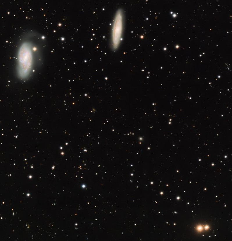
R. Q. Fugate and J. W. Briggs sent out a lovely photo of the Leo Triplet of galaxies, a section of which is displayed below. When looking at such photos with their profusion of stars, my eye tends to single out pairs of stars, and I have often wondered whether the stars were actually close, gravitationally bound, or whether my eye was fooled by randomness. Take, for example, pair of bright orange stars in the lower right corner. Are they close to each other?
Beginning with M66, the galaxy on the left, one can hop down to the bright pair using, say, Simbad (http://simbad.u-strasbg.fr) and its Aladin viewer. These stars are identified as HD 98172, the brighter one, and BD+13 2382. From their coordinates, one sees they are further apart than most double stars, over 2' or about 136 arcseconds east-west as a first estimate, and so are unlikely to be related.
Nevertheless, both Regulus and Iota Leonis in the same constellation have companions listed in the Cambridge Double Star Atlas with separations of 2.9' and 5.5'respectively. So it might still be conceivable the stars are conjoined by gravity. The Simbad also gives proper motion, radial velocity and parallax data for each star. These data indicate the two stars are headed in different directions at different speeds and, by parallax, are at quite different distances from us. So these two stars, however alluring, form an optical, not a physical pair.
posted at: 16:14 | path: | permanent link to this entry
Wed, 15 Apr 2020
Telescope Clock Drive Motors
After near 20 years there is time for astronomy. Two telescope mounts purchased in Michigan have right ascension drives powered by electric motors.
The oldest motor, which came with a Discovery 8 inch Newtonian, has four leads and runs off 12 volts DC. My initial assumption that four leads meant it was a stepper motor proved wrong. There is also the possibility a separately excited DC motor where rotor and stator are powered separately. Such motors can maintain constant torque at different speeds, and the hand controller that came with the drive provides up to six different speeds.
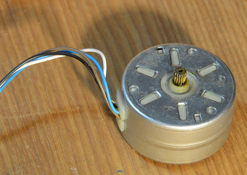
These things came to light because the clock drive had stopped working. I blamed the controller and then the motor as I tried to replace the controller with a Phidgets stepper motor controller, all to no avail. Meanwhile I had sprayed a carburetor cleaner into the gearbox trying to loosen up the old grease. The cleaner container contains acetone which disolved the gearbox casing thus providing access to clean the gears. With freely turning gears, the clock drive works as it should.
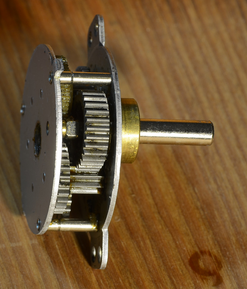
Nevertheless, this motor really is a stepper. And I was finally able to control it with an EasyDriver stepper driver connected to a Beaglebone Black. It's a little unusual though with 48 steps per revolution where 200 steps is typical.
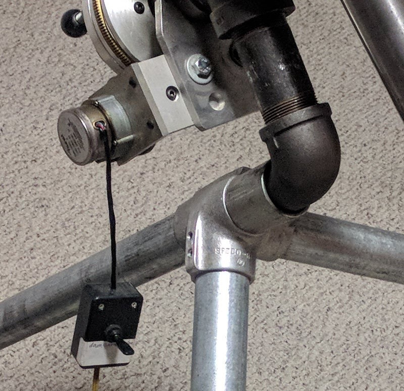
The second motor, which came with a pipe mount purchased from a basement machinist shop near Livonia, MI, runs off 110 volts AC. This unassuming motor, which I initially mistook for a cheap toy, is a synchronous motor, and is still available even today from Hurst electronics for over $100. These motors have the property of maintaining a constant speed under increasing loads. This came to light because I blamed the motor when the mount failed to track accurately and I searched for a replacement. It turned out that backlash was the culprit and the motor was performing as it should have.
posted at: 17:47 | path: | permanent link to this entry
Sun, 08 Apr 2018
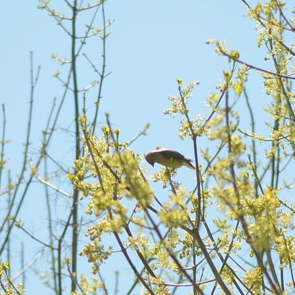
Cedar Waxwings Eating Tree Flowers
Along the creek bed behind our warehouse next to a cottonwood tree stands a multi-stem tree with shallow furrowed bark like this:
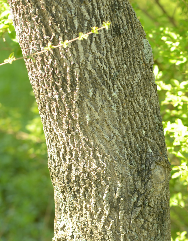
Leaves still in bud and flowers like this:
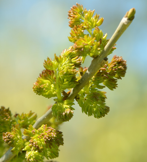
A small flock of cedar waxwings were busily eating the flowers it appeared:
posted at: 21:25 | path: | permanent link to this entry
Sat, 09 Apr 2011
King Snake Crawl By
A short walk up our street brings one to an overlook of the Galleria, Alabama's largest indoor shopping mall. But an equally short walk in the other direction leads to houses nestled among the woods along Patton Creek. This finger of nearly natural land brings us the occasional wild visitor: armadillo quads, coopers hawks, deer. Last week JY found a young black king snake nearly underfoot.
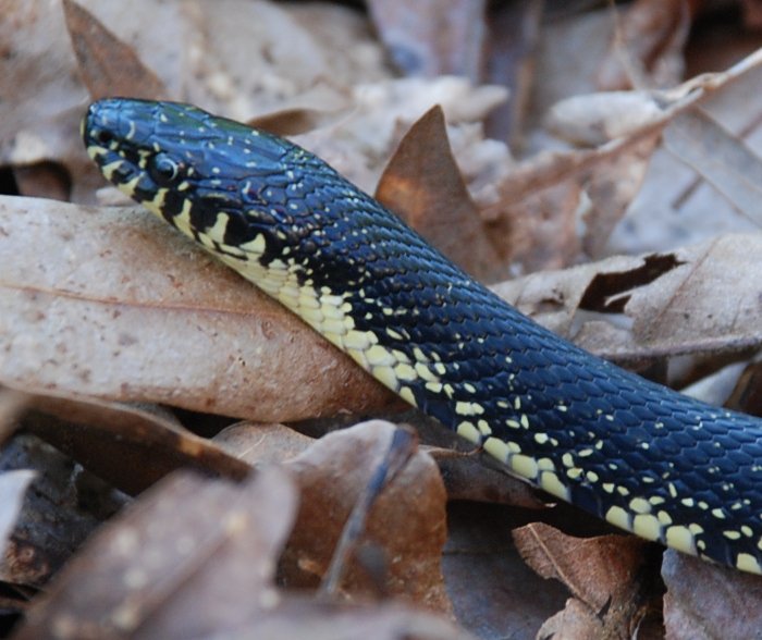
It was about 18 inches long and quite small in diameter as you might infer from the size of the oak leaves in the litter around it. It did not seem to be frightened and allowed the camera to come quite close in.
posted at: 23:05 | path: | permanent link to this entry
Sat, 05 Mar 2011
Primitive Melt Cutter
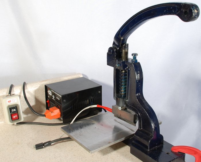
Last year one of our suppliers sent us a simple tool to cut the webbing we buy into the canvas belts we sell. A cartridge heater is fixed in the blade which, when hot, will cut and seal webbing made from synthetic fiber like polyester or nylon.
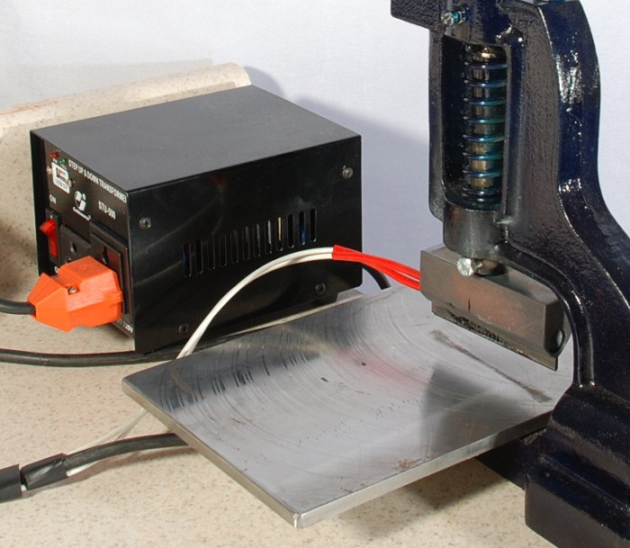
To work properly, the cartridge needed a 220 volt power source. The diameter being metric seems to narrow the market in cartridges to 220 volts, but no matter, I found a 110 V to 220 V transformer on-line--cheap and a lot easier than wiring in two out-of-phase circuits! A little bit of grease and the arm brings the blade down to the anvil quite easily. A strong spring pushes the blade back up.
Automated cutting machines are comparatively inexpensive, $3000 plus ex factory in China or Taiwan. I don't know how long it will last, but this hand tool tickles my fancy and cost less than $100.
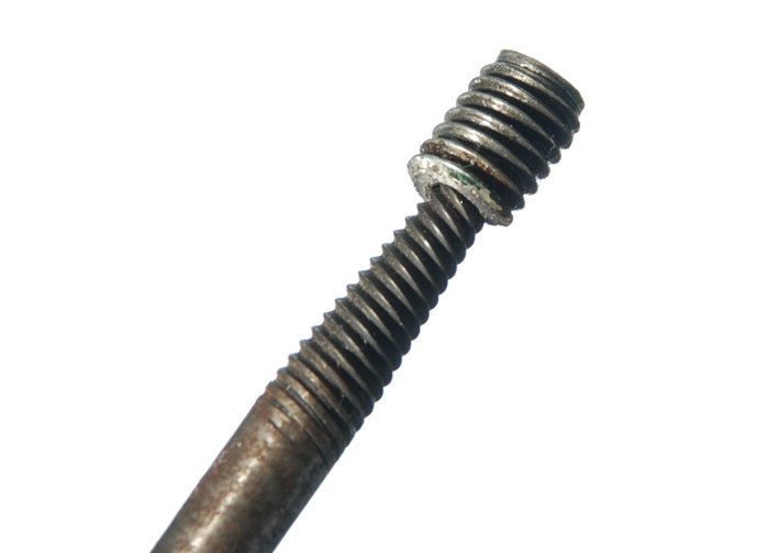
There was only one glitch. The head of the bolt that fixes the hot blade in its socket snapped off. Luckily, I had the right tool, a bolt extractor. It had lain unused in my tool box since the time M. Carpentier helped me rebuild the engine of my 1959 Volkswagen some thirty years ago.
posted at: 23:02 | path: | permanent link to this entry
Tue, 22 Feb 2011
Connections
My kind brother Tom, sent me a recording of Michael Daugherty's "Deus ex Machina" for piano and orchestra, the title referring not to a ruse in drama but to trains. According to Daugherty's notes the third section was inspired by the photographs of trains from the late 50's by O. Winston Link.
I wasn't familiar with Link, but I did meet a photographer who followed trains in the same era, Ted Rose. Ted Rose followed and photographed trains in Illinois, Mexico and Guatamala in the late 50's and early 60's. I met Ted through his wife Polly, who was Dr. Wiegle's secretary at St. John's College where I attended in the early 70's. Polly was a friend to me, and many members of the college. You need only see the picture of her here to understand.
I as at the Rose's one evening, (a beautiful house, by the way, that Ted and Polly had built themselves), and when Ted mentioned his youthful adventures as a train photographer, I was fascinated, and bought one of his photographs to take home to my parents. My mother framed it and saved it and I have it now:
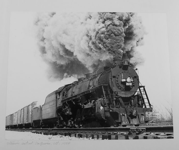
This was taken in 1958 according to Ted's notes at the bottom; he would have been 17 or 18 at the time. If this photo seems to lack distinction, jump over to www.railroadheritage.org and you will see Ted was very good.
I might have thought my father would like the photograph because he had lavished such care on the Lionel trains he bought for us as children. I still have these, too. Here is one, probably from 1956 or so:
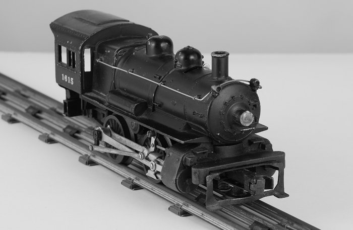
And the music? Not wistful as you might expect from a look back; more a driving, rhythmic sound poem. Worth a listen.
posted at: 23:30 | path: | permanent link to this entry
Sun, 13 Feb 2011
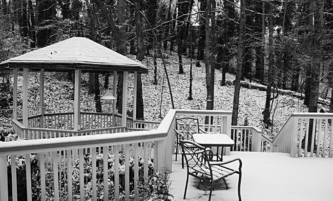
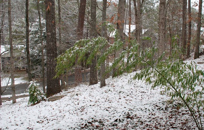
Alabama Snow Storm
February snow in Birmingham.
posted at: 23:14 | path: | permanent link to this entry
Fri, 21 Jan 2011
Preparation
In my previous post I showed a cabinet top I bought a Home Depot for $4.13. Today JY and I built a wooden stand for the cabinet to sit on, making an inexpensive work bench. Four 2 x 4's and a piece of plywood, cut and screwed together. Humble, I know, but fun.
It put me in mind how my brother, John, loved carpentry from early on, and how, contrary to what kids with college ambitions were supposed to do, he took "shop" in junior high. His project, an end table, sat between the twin beds in our bedroom long after all the kids had grown and gone.
Some years after graduating from college, John bought a decrepit house and remodeled it in a grand way. Both he and my mother are pictured below in the finished product. One can glimpse his work with the cornices, the book cabinets, the fireplace mantel, the over-the-top kitchen in the background.
In digging through old family photos trying to find some record of John's carpentry work, I came across an old Artesia Daily News clipping where John and one of the Watson boys were pictured for having won prizes in the state science fair.
Like taking shop, John also took shorthand in high school, probably the only boy in the class and surely the only student with college in mind. When he did enrol in engineering studies in 1972, he recorded the professors' every word and transcribed it longhand back at the dorm later. He did very well in school that year.
It amazes me now to think back on all that.
posted at: 22:01 | path: | permanent link to this entry
Thu, 13 Jan 2011
Measuring Webbing
A problem we have needed to solve in our webbing distribution business has been to find an economical and relatively fast method to measure out and cut given lengths of fabric. This method should be designed to minimize repetitive stress on the hands and arms of the operator.
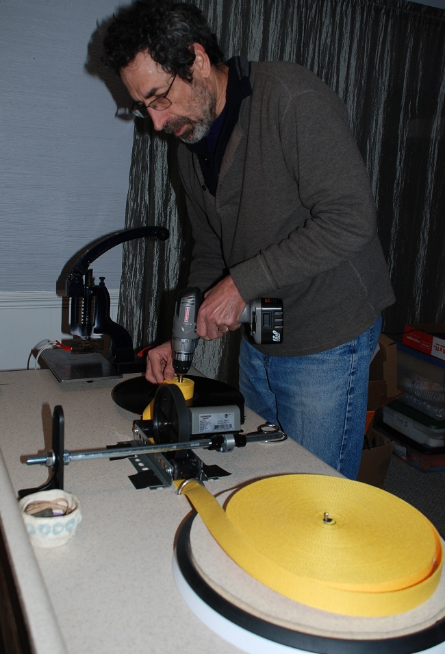
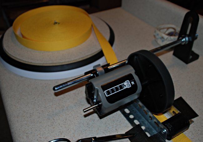
A first shot is pictured in the table below:
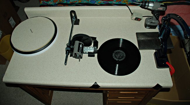
The table surface is a plastic laminate counter top on sale at Home Depot for $4.13, one piece of which was cut out and set into the inexpensive lazy susan on the left. The turntable on the right is constructed from a lazy susan frame with skid pads and a round piece of plywood attached. Stealing a page from Dobsonian telescope instructions, the plywood is topped off with Bing Crosby Christmas carol LP, a recessed hex screw bolted down in the center. A measuring meter is set in the center with angle iron, tape gun rollers and U-bolts for guides. A melt cutter is on the right.
To cut a 30 foot roll from a larger roll, we mount the source on the large lazy susan and thread the webbing though the meter. Then we reset the meter and squeeze the lead between the driver bit and a post on the LP. Squeaze the variable speed driver and away we go.
posted at: 11:06 | path: | permanent link to this entry
Tue, 04 Jan 2011
The printing press and the internet.
A chapter in "Radical Enlightenment" by Jonathan Israel reminded me of the unfolding story of censorship of the internet in China. The chapter, "Censorship and Culture", recounts the efforts by religious and secular authorities in Europe to suppress erotica, philosophy challenging religion, and undesirable political opinions during the years 1650 to 1750.
The problem for the churches and governments was the printing press and transportation. Books were printed in many different locations, often surreptitiously, and smuggled across borders. Similar, it strikes me, to the difficulty faced by the Chinese government to control, not just a Google, but hundreds of millions of individual citizens.
Of course, there is no reason to think culture will evolve in China as it did in Europe, but it is interesting to think that the freedom to form ones own opinions and to say, even publish, what one opines was not always a western value. Even enlightened opinion felt the state should defend morals and religion. Intellectual freedom and freedom of the press were radical ideas in Europe during the century. Suppression of the atheists seemed as acceptable to most seventeenth century Europeans as the imprisonment of Liu Xiaobo does to the Chinese today.
posted at: 23:02 | path: | permanent link to this entry
Thu, 24 Dec 2009
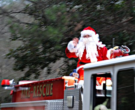
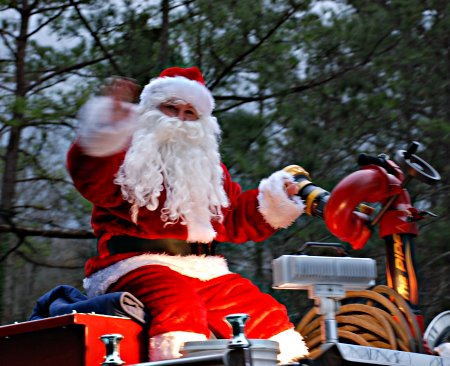
Santa Comes By
Every year in Hoover, AL, Santa hitches a ride with the fire department
and winds his way down every street in town, waving happily to all that
come out to see him, much to the delight of the neighborhood children.
posted at: 16:45 | path: | permanent link to this entry
Mon, 25 May 2009
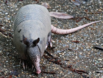
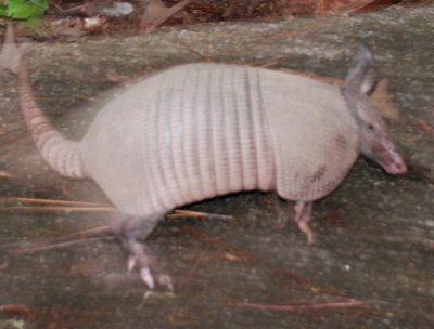
Armadillo Quads Pay a Call
An armadillo litter, four homozygotes, dropped by our woods for some grub a couple weeks ago. They were probably holed up on the banks of Patton Creek nearby. JY kept snapping photos, but they were oblivious til suddenly one noticed her and, characteristically, jumped. Startled, JY did the same.
posted at: 23:08 | path: | permanent link to this entry
Sat, 10 Jan 2009
Surround Soft Box
Providing diffused light for small reflective objects (mostly belt buckles for me) was a difficult photographic problem for me. My friend Ben B. recommended a cloud dome, but they list at $200. I finally hit on an inexpensive construction suggested by D. Montizambert in Creative Lighting Techniques.
I cut a 40% sector of a 32 inch radius circle from a sheet of white woven nylon. Sewing the sector along the two radii forms a cone, and sewing a piece of clothes-line wire along the 72 inch circumference provides a frame for the cone. Cutting the tip provides a hole for the camera lense. Usually, I hold it on the lense body by hand, but with a rubber band, one can free his hands. Mounting the camera on a tripod as shown, while not necessary, is also useful for maintaining fine control.
I use two monolights, one one either side of the cone. The flexibility of the cone lets me place the reflection of the lense from a convex mirror pretty much where I please.
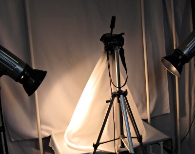
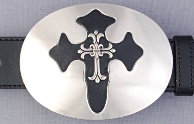
The buckle below illustrates the diffusion of light from the set-up above. While not hard to do in this case, the lense reflection is hidden by the buckle inlay.
posted at: 17:00 | path: | permanent link to this entry
Sun, 28 Dec 2008
American Crafts
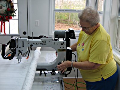
This Christmas we caught a fleeting glimpse of the state of American quilting. Joanne T. has worked in photography and various crafts for many years. In the past three years, she has taken up quilting. Quilting is an entire universe with a history of patterns, a large network of quilters, and many levels of accomplishment.
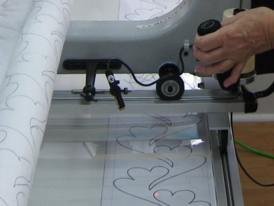
This month Joanne upgraded her quilting machine. Pictured below, this machine can sew quilts up to ten feet wide. Except for binding the edges, it performs the last step in the quilting process, sewing front and back sheets together with the batting in between. The operator can follow a pattern using a laser guide as Joanne is doing in this picture (see the detail below). Or the operator can sew free-hand, in which case the handles on the opposite side of the arm would be used.
A quilt finished with her previous machine is shown in the next picture (along with her granddaughter, to whom she gave it).
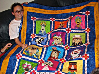
Joanne lives on a small farm in Washington Parish, Louisiana, and sustained major losses in Hurricane Katrina three years ago. As we were about to leave, she pointed across a pasture to the woodlands. The new green growth underneath the sparse canopy of mature trees represented seedlings germinated from the seeds of trees destroyed by Katrina. This is just visible in the background of a photo I had taken earlier (see below).
I see an analogy in this. Just as new seed sprouts after Katrina, there is a resurgence of skilled activity in the land where the once proud textile industry was laid low by globalization.
posted at: 14:36 | path: | permanent link to this entry
Tue, 17 Jul 2007
Lake Victoria and Sauper's film
We saw Darwin's Nightmare on DVD this past weekend. We watched it twice and watched the interview with Sauper as well. It seems to have generated some controversy. Wikipedia provides some information there.
Sauper explains he is being indirect, but I think his focus is on the effects of globalization and the arms trade on the people in undeveloped, poorly governed countries. The use of Darwin's name is a little misleading; his interest lies not in natural science, but politics, "Social Darwinism" as he says in his interview.
Nor does economics play a large role. Numerous times his subjects note/claim the jets carrying the fish to Europe arrive empty, and numerous times he asks whether they might not actually bring munitions.
What he presents is devasting, especially the cycle of aid to factories to dislocation of workers to public health collapse. But I'm left desperately curious. What is the train in the background transporting? Where do the fish factory owners and workers live? The street urchins are dressed in rags; where are the tee-shirt vendors? How does cash get from perch to arms?
Sauper makes a very good point in his interview; the images he captured were not easily obtained. It was difficult to transport cameras, to get access to airports, even to follow the fish carcasses. Another demonstration of how much we wouldn't have known without serious effort, and, by inference, how much we do not yet know.
posted at: 11:06 | path: | permanent link to this entry
Sun, 01 Jul 2007
Texas tee in Hispaniola
A couple years ago, I mentioned The Travels of a T-Shirt in the Global Economy and how Texas-style cotton farming extended past the Llano Estacado into the Pecos Valley where I grew up. This year I caught a glimpse of the end of the tee-shirt life cycle described in Pietra Rivoli's book.
My son is studying at the University of Miami medical school. For his spring break this year, he went to the Dominican Republic to help out in clinics and learn. He has described some of his experiences there in his on blog, philcopper.com. Here is one of the pictures he brought back

Rivoli describes how the tee-shirts that Americans discard get bundled up and shipped to Africa and sold in small stands there. But of course there are many destinations for America's used clothing and the young medical student pictured seems amused with this small incongruity.
posted at: 20:50 | path: | permanent link to this entry
Addendum and second thoughts on photographing olive green
When I first looked at the difference between actual and theoretical values of red in the "moderate brown" square of my color checker, I just assumed that the 18/256 difference was perceptible. I should record that difference:

The problem is that on my consumer grade CRT monitor, the actual recorded value appears closer to the card in my hand illuminated either by indirect sunlight or by the Solux halogen light in my study.
Maybe my card is off? Maybe the reflectivity of the fabric under my static light sources is somehow missed by the camera in flash lighting? And I am mistaking some other difference for color difference?
posted at: 18:44 | path: | permanent link to this entry
Wed, 27 Jun 2007
Trying to get colors right in photography
Over the last couple of years or so, there have been a number of fabric colors that I just never seem to capture. Today I just want to make a note of my attempts to reproduce the olive green that some of my military web belts exhibit.
First step: setting the white balance on my camera. I have a Nikon D-50, and I set the white balance by photographing an 18% gray card.
Second step: including a color checker in the photograph of the fabric:
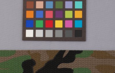
In this photograph, exposure was chosen that seemed best to reproduce the color checker as a whole. Also, the grays correspond pretty well to the values for sRGB at brucelindbloom.com. My 2 high and low values are spot on and the middle two are high by 13 (out of 256). Measurements of the image of the color checker were taken with GIMP's color picker.
My own problem with this photo is that it seems to change the olive drab to a brown drab. The problem can be seen in the color checker in the first spot; the "dark skin" or "moderate brown" have listed sRGB value of (115, 80, 64) while the photograph above reads (139, 77, 57). There is too much red in the medium brown. Using GIMP's color curves to tone the red down around the value of the olive green in the belt does improve the color reproduction of the olive green--but, of course, throws the greys out of whack.
It is also curious to me that the other related color, "foliage" or "moderate olive green" is pretty much in line; (88, 113, 64) in the photo and (88, 108, 65) in the chart.
I can only conclude the problem is in the camera (or the camera software).
posted at: 23:47 | path: | permanent link to this entry
Sun, 03 Jun 2007
Using extension tubes to photograph a fossil
Recently I visited the photo store to shop for a macro lense for my Nikon D-50. The camera is a paradigm of sophisticated technology modern manufacturing has put within reach of someone of modest means. The Nikon macro lenses have not followed suit (yet), the least expensive costing more than the D-50 body. So I purchased a 12-20-36mm set of extension tubes for $150. Surely I need not have spent so much--Rick at Shutter Freaks reports paying half as much for his Canon--but you are paying for more than the product when you go to a camera shop...
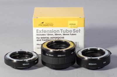
The benefit of the extension tube is to allow the lens to focus on closer objects without significantly changing in angle it subtends, thus increasing the angular magnification. Wikipedia has more detail. The downside is that the lens cannot focus on distant objects. Furthermore, built-in calibration of a zoom lens that keeps an object in focus while zooming no longer works, of course. Also a longer extensions and shorter focal lengths, the distance between the nearest and farthest object that can be brought into focus becomes so small as to make focusing difficult. But, hey, a microscope is useful with a narrow range of focus andwithout the capacity to focus on distant objects.
For my own records, at least, here is ranges I get for the Nikkor AF 70-300mm set at 70mm. Distances are approximate (precise to 1/8") and are what I measured between the focal plane mark and the object. At some point between the 20mm and 36mm extension, the minimum and maximum distances invert with respect to extending or retracting the objective lens!
| Lens retracted | Lens extended | |
|---|---|---|
| no extension | 60" | infinity |
| 12mm extension | 22.125" | 24.125" |
| 20mm extension | 18.875" | 19.25" |
| 36mm extension | 15.375" | 14.75" |
To illustrate, here is a wonder fossil picked up by Bill Haywood, forester, author and rock hound extraordinaire. He says this about it:
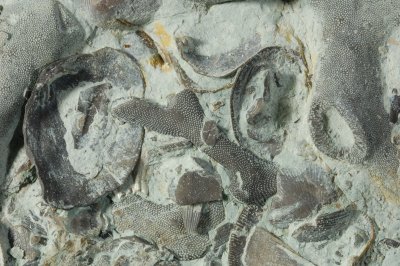
This is out of the ordovician era. Corals were just barely evolving. The main fossil in the center is a branching coral and some researchers think that it might even have been a sponge but we are sticking with branching coral. Most of the other fossils are brachiopods. This deposit was made about 500 million years ago. The layer you are looking at is blanketed by limestone so the ocean must have receded and this was a clay deposit in a delta area. How about the detail on those fossil surfaces!?The area from the 12mm extension is about 4" by 2.625":
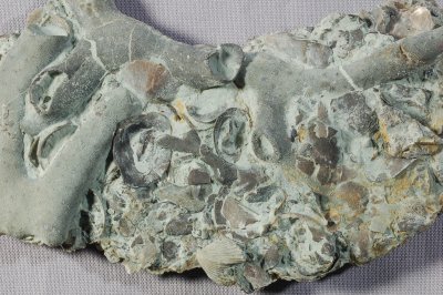
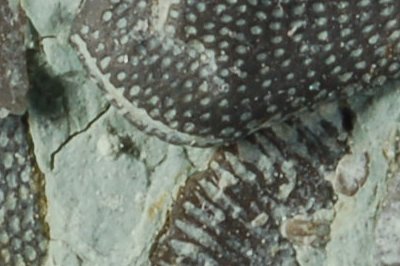
and the area from the 36mm extension is about 1.75" by 1.125":
Finally, here is a pixel-for-pixel detail from the previous shot:
posted at: 16:00 | path: | permanent link to this entry
Tue, 29 May 2007
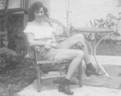
Andrew Wyeth revisits Kuerner's farm
Nearing 90, Andrew Wyeth revisited Kuerner's hill to paint Margaret Kuerner's portrait this year. Blind and confined to bed, now close to 90 herself, she has lived at the foot of Kuerner's hill, across Ring Road from the Kuerner farmhouse for over fifty years. So that famous knoll is more than a fanciful background, it is the view from Margaret's window.
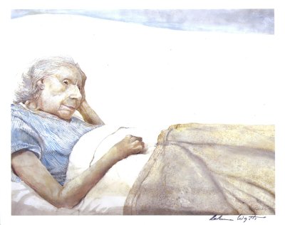
Wyeth, like any artist, I suppose, has his own intentions, and Wyeth himself has often exhorted his viewers to look beyond the image, and perhaps the juxtaposition of his icon and reflective denizen gesture towards a retrospection of his own. But Margaret's serenity is not Wyeth's creation and is no accident of time. She was gentle before and her memory is clear. When I mentioned the photo to her, she chuckled at the memory of Palm Beach and her own youth before coming to Kuerner's.
posted at: 09:53 | path: | permanent link to this entry
Mon, 03 Apr 2006
Halogen light stand for studio photos
Getting accurate colors of the products I photograph for my website has been a constant struggle for a novice photographer like me. I feel I've made real progress for a modest investment following a wonderful article over at creativepro.com.
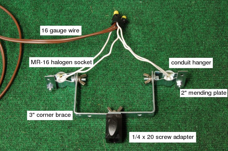
Figure 3 in this article plots the spectral power distributions of special "daylight" fluorescent lamps and of filtered halogen lamps against the D50 referent. I found that using "natural sunshine" fluorescent bulbs and calibrating the white balance of my Nikon D-50 to a gray card solved the problem I was having representing various olive greens. Needing directional lighting and seeing how filtered halogen achieves a color rendering index of 98 or 99, I decided to try making my own halogen fixture. The parts I have bought are
- Smith-Victor 1/4 x 20 screw adapter for light stand
- Provides a screw stud for attaching a light assembly to one of their light stands.
- 2 3" corner braces
- From the hardware store, these "L" brackets provide two vertical mounts as well as horizontal angle adjustment. They're tightened down with thumbscrews for convenient adjustment.
- 2 3/8" conduit hangers with speed thread
- Instead of conduit, the hanger holds a halogen light socket. I used a 1/4" x 3/4" serrated flange bolt to attach the hanger to the "L" bracket and tightened it with washers and thumbscrew to facilitate vertical angle adjustment.
- 2 2" mending plates
- These are attached to the hanger clamp bolt by two hex nuts and provide a handle for vertical adjustment of the lights--I expect the clamp to get too hot to handle comfortably.
- 2 MR-16 sockets
- The filtered halogen bulbs (Solux) I need have an MR-16 base--one reason I couldn't use off-the-shelf fixtures I saw at the hardware store.
- 1 120VAC to 12VDC transformer
- Halogen lights use DC current. I'm expecting to use 2 50 watt bulbs but I spent an extra $10 for the 150 watt transformer just in case I need more wattage later.
- 1 6' cord set with switch
- This one came with a socket at the end, but I cut it off and spliced the cord to the transformer.
- 7' 12 gauge wire
- I'm planning to let the transformer rest on the floor, so I need a length of heavy guage wire (because of the high amperage) to run from the floor to the top of the light stand.
Here is a photograph (click to enlarge):
posted at: 09:41 | path: | permanent link to this entry
Thu, 23 Mar 2006
Dr. Bergren talks to Kiwanis about breast cancer
Dr. Carl Bergren spoke to his Dearborn Kiwanis Club last night about an apect of his surgical practice. I, myself, at my son's recommendation, have been slowly making my way through Atul Gawande's Complications: A Surgeon's Notes on an Imperfect Science. The combination induces a disquiet that, I suppose, accompanies any meditation on our mortality, but there is also an exhilaration at gaining a new perspective on a familiar topic, the practice of medicine.
It is easy to forget how we deal with the world largely through abstractions, and it is easy to forget how difficult and fallible is the process of abstracting from experience. In fact, religion and other human behavior show how abstraction can be distasteful as well as difficult. Surely there is no better example of the jarring confluence of shamanism and science than the medical profession.
Not to put words in his mouth, but Dr. Bergren seemed to feel from his own experience that the increasing incidence of cancers is environmentally related, but at the same time seemed overwhelmed by the difficulty of distinguishing which of the many changes in our environment might be most harmful. He mentioned a population in Japan which exhibited one of the lowest breast cancer rates, but then said when members of that population are removed from their location and diet, they quickly exhibit the same rates of cancer incidence as their new group. (You can imagine how difficult it would be to establish even that one simple statistical fact!) He speculated that the reason might be related to the high consumption of soy products in the Japanese population.
On the other hand, he did mention that there appear to be differences in cancer incidence among racial groups. When questioned further, he said that african-americans tend to exhibit more aggressive forms of breast cancer, but when asked whether that fact might be due to differences in diet and environment, he said only that the issue was a contentious, even political, one. Again, think how difficult a statistical question is being asked. It is hard enough to relate race to genome and near impossible to tease out factors of diet, culture, access to and practice of healthcare.
Another suspect environmental factor Dr. Bergren mentioned several times was growth hormones passed to us through meat. Although he allowed no connection between breast size and cancer rates, he did say that through the years of his practice he felt that there had been an increase women's breast size on average. He didn't seem to feel it was related to obesity, but rather allowed his suspicion to rest on environmental factors like growth hormone. When pressed on this question, shouldn't there be some statistically testable aspect of his hypothesis, he only commented on the difficulty, observing how the similarity of human and synthetic growth hormones fed to livestock made it impossible to relate even the levels of hormone-related chemicals to meat intake.
After considering the difficulties of medicine, Dr. Bergren mentioned the book Doctors Never Lie with which I a not familiar, but he certainly put me in mind of one with which I am: How to Lie with Statistics. And, as I often do, I felt amazed how humans were ever able to abstract anything useful from the morass of physical experience.
posted at: 09:39 | path: | permanent link to this entry
