Two Infinities
Wed, 01 May 2024
Speckle Interferometry Background and Example
Presented to Enchanted Sky Star Party October, 2023.
Light
Astronomers study light.
wave propagation
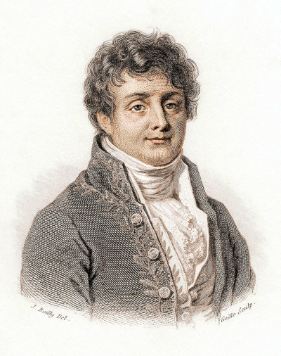
Christiaan Huygens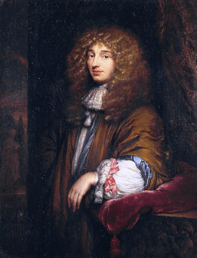

superposition
Thomas Young diffraction and interference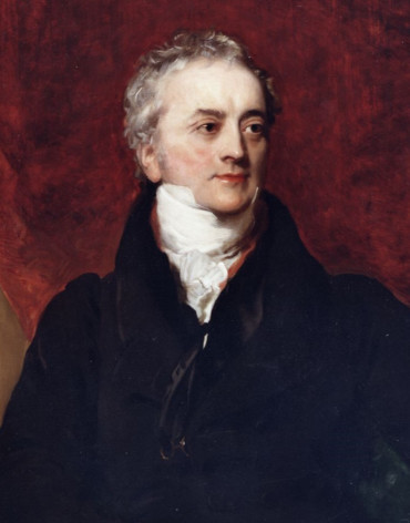

(painting by Henry Perronet Briggs)
speed of light differs with media
The different media might be different densities of air. Different speeds lead to refraction (Fermat's principle).
Pierre de Fermat
Laser refracted by ultrasound

Poisson's spot
Arguing against Augustin Fresnel's wave theory of light, Siméon Denis Poisson claimed there would have to be a tiny bright spot in the middle of the defocused image of a star in a telescope with central obstruction. When, contrary to Poisson's expectation, such a spot did occur, many scientists were won over to the theory. (Image from Suiter's "Star Testing".)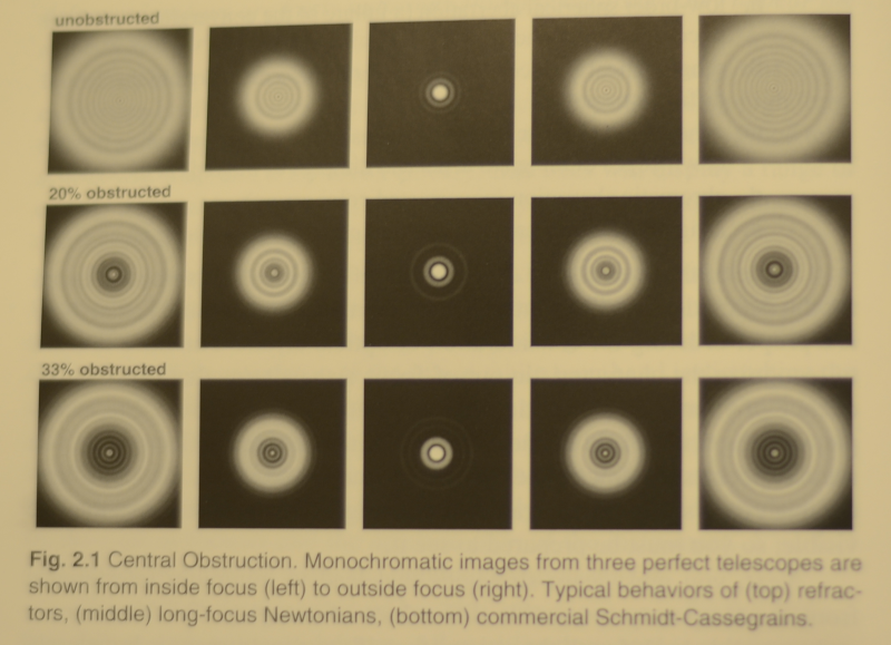
X-ray chrystalography
The periodicity of electro-magnatic radiation is useful for delineating the periodic structure of chrystals -- most famously for uncovering the structure of DNA: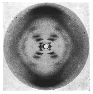
Basic Idea
Same Image Viewed Two Different Ways
Joseph Fourier proposed that any function can be viewed as the superposition of cyclic functions. For example, instead of viewing an image as an array of pixel values, view it as a superposition of waves. If a good approximation of the function can be obtained with a few waves then the change of point of view reveals structure.
![]()
Averaging Out Atmospheric Turbulence
Antoine Labeyrie thesis, extension of Fizeau and Michelson's interferometer methods:

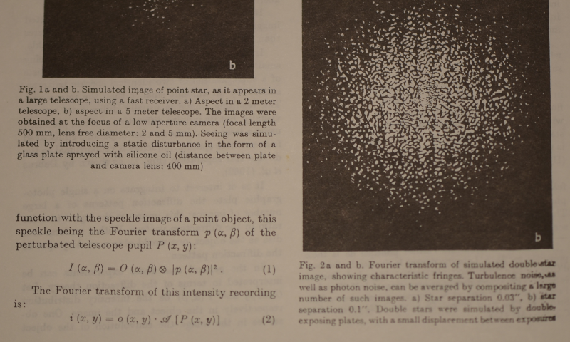
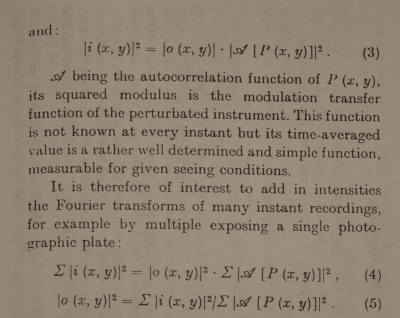
Quote: "Speckle" refers to the grainy structure observed when a laser beam is reflected from a diffusing surface.
Labeyrie snippets courtesy J. Briggs' book from Yerkes library.
Binary Star Example
cou1333: Constellation Cygnus, Tycho2 2702-00556-1
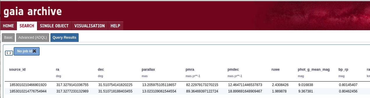
From parallax the distance from Earth is about 247 light years. From ruwe each star probably has a companion; that is, this double is probably physical.
Go to Astropy to compute the angular separation between Gaia coordinates.
#!/usr/bin/env python3
import sys
import astropy.units as u
from astropy.coordinates import SkyCoord

# usage: angle_sep.py 〈ra1 〉 〈dec1 〉〈ra2 〉〈dec2 〉 (in degrees)
# output: angular separation in arcseconds
ra1 = float(sys.argv[1])
dec1 = float(sys.argv[2])
ra2 = float(sys.argv[3])
dec2 = float(sys.argv[4])

c1 = SkyCoord(ra1*u.deg, dec1*u.deg, frame='fk5')
c2 = SkyCoord(ra2*u.deg, dec2*u.deg, frame='fk5')
sep = c1.separation(c2)
print('angular separation',sep.arcsecond)
Run the script like this:
./angle_sep.py 317.3279141036755 31.510754141820225 317.3277233132989 31.510718188403455Get the result in arcseconds:
angular separation 0.599698853444346
Pixels to Angles
Getting from pixels to arcseconds.
Using Plate Solve
Using astrometry.net solve-field, the plate solution for this image: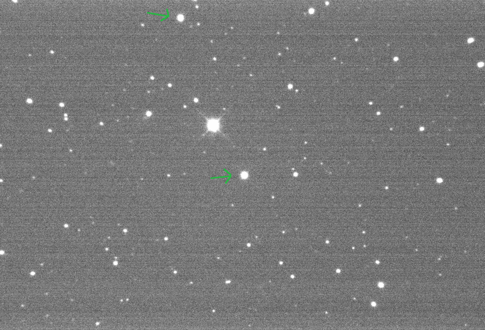
provides both pixel location and sky coordinates of two brighter stars on opposite sides of our target, cou1333. Then astropy SkyCoord.separation computes the angular separation, 211.88567303817118 arcseconds. From the pixel coordinates of the indicated stars, the separation in pixels is 727.43897225043697365183 px. So the telescope + camera with 4x4 binning comes to .2913 arcseconds per pixel, .0728 arcseconds per actual pixel.
Using a diffraction grating
This diffraction grating has period d = 15.17 mm: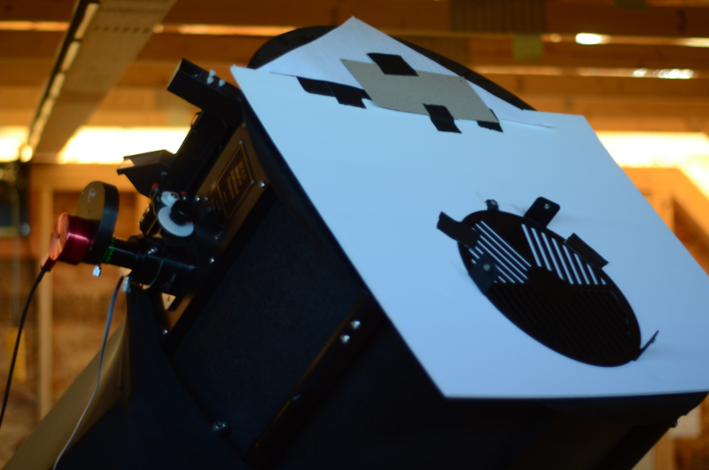
Pointing the telescope at Sirius with this mask and an Hα filter:
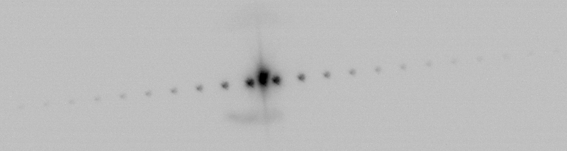
The diffraction grating formula says sin(θ) = λ/d.
With λ=0.00065628 mm, θ = .00004327 radians or 8.925 arcseconds.
The distance of the first spot from the central spot is estimated at 31.14 px, so this route yields 0.2866 arcseconds per pixel, slightly less than the plate solve approach.
cou1333 images
Our goal is to extract a separation measurement (ρ) from 200 exposures.
raw images
Here's one: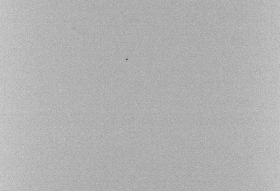
Field of view: 10'x7'. Exposure: 1/100 second.
signal to noise
Zooming in to get a feel for signal to noise (SNR):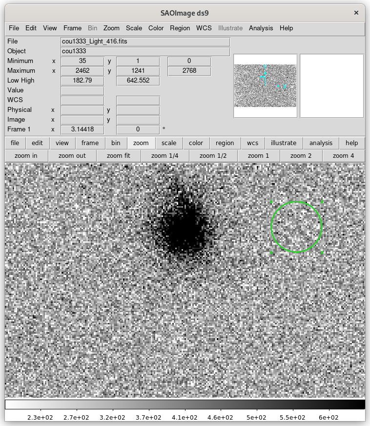
The average intensity in the 862 pixels around cou1333: 778 counts
The average intensity of sky: 339 counts
SNR sample: 2.3
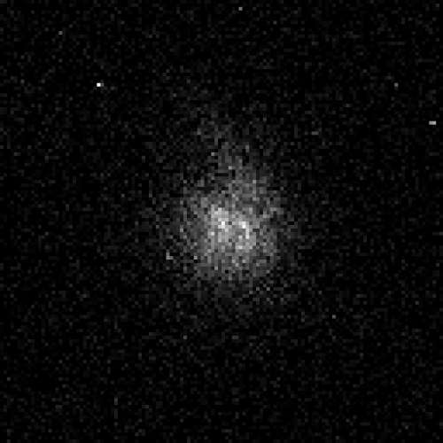
Extracting a region of interest
We average each pixel with its immediate neighbors and extract a 128x128 subframe around the brightest one. Here's the first one: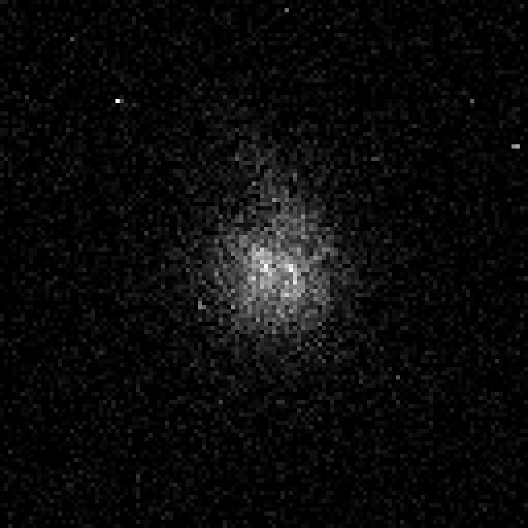
Jumping to SAO ds9 fits image viewer...
Fringes
Following Tokovinin, Mason, Hartkopf "Speckle Interferometry...", 2010, implementation of Labeyrie (as best I can).- Compute the power spectrum of each image
- Compute average of power spectra
- Filter noise
- Divide by best guess at MTF
- Fit model to fringe
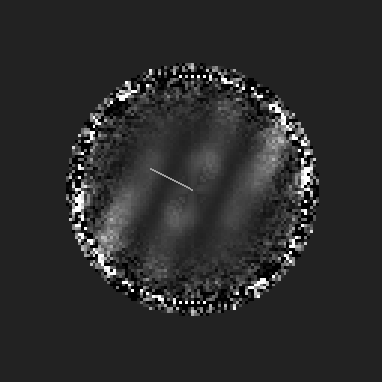
Distance from center to peak of fringe ~16 px corresponding to a plane wave with period 128/16=8 pixels.
Using angle subtended by a pixel = .0728 arcseconds, multiply by 8 and get .5824 arcseconds.
posted at: 14:57 | path: | permanent link to this entry
